Analysis of Journey to Work Travel Behavior by Car and Bus in the
Sydney Metropolitan Region
Suthanaya, P.A.1
Abstract: Car dependence is a fundamental problem in the sustainability of cities with low-density suburban sprawl. Increasing the use of public transport is one of the policy objectives commonly adopted to overcome this problem. It is essential to study journey to work travel behavior by car and bus. This paper applied preference function to analyze travel behavior and Moran’s I spatial statistic to evaluate the spatial association. The results indicated that the commuting preferences of residents have moved towards distance maximization. In general, bus was preferred for shorter distance trips whilst car was preferred for longer distance trips. Unlike car, by increasing distances from the Central Business District, residents tended to use bus for shorter distance trip. A significant positive spatial association was identified for both the slope preferences by car and bus where zones with a preference towards longer or shorter trips tended to travel to zones with similar preferences.
Keywords: Travel behavior, car, bus, spatial association.
Introduction
The internal structures of metropolitan regions have changed. Decentralization of employment towards the outer areas and suburbanization of residential areas with lower population densities has arguably increased car dependence. This condition has negative effects, among others; lost time and productivity, vehicular accidents, greenhouse gas emissions, deteriorating air quality and associated risks on respiratory and cardiovascular health [1]. Evidence in Australia, and other countries, suggests that urban form is a significant factor in car dependence [2].
The reduction in Vehicle Kilometer of Travel (VKT) is one of the policy objectives adopted by many cities in order to achieve environmentally sustainable transportation. Intuitively, a more convenient location of employment relative to housing is expected to reduce the length of trips. Several studies argued that distance from the Central Business District (CBD) influences travel behavior. Empirical study conducted by Yang [3] indicated that decentralization was followed by different transportation outcomes. The academic literature on the impact of urban form on travel behavior has increasingly recognized that residential location choice and travel choices may be interconnected [4].
1 Department of Civil Engineering, Faculty of Engineering,
Udayana University, Bukit Jimbaran, Bali, INDONESIA Email: [email protected]
Note: Discussion is expected before June, 1st 2011, and will be
published in the “Civil Engineering Dimension” volume 13, number 2, September 2011.
Received 9 April 2010; revised 24 September 2010; accepted 28 October 2010.
Improving the quality of urban public transport is one of many strategies proposed to improve mobility options and to address car dependence [5]. However, Holmgren et al [6] identified that local public transport development in many European countries, has for a long time been on the decline. In developing country, Joewono and Kubota [7] stated that paratransit has an important role in providing feeder service to public transport user that has to be considered. According to Mulley and Nelson [8], public transport should be demand responsive. Therefore, it is important to understand factors influencing commuting preferences by public transport.
change in urban form over time at the zonal level [12]. However, it is quite difficult to find historical data where significant change in urban form followed by significant change in travel behavior. During 1981 to 1996 period there had been significant change in urban form and travel behavior in Sydney, Australia which was caused by massive decentralization. Using journey-to-work (JTW) census data over a 15-year period (1981 to 1996) in Sydney, this paper applies preference functions to study the journey-to-work commuting preferences by car and bus. The objectives of this study are: to analyze the stability of commuting distance preferences by car and bus of the Sydney’s residents and to analyze spatial association of the slope preference functions among zones.
Literature Review
Theory of Preference Functions
Preference function is an aggregate of individual travel behavioral responses by a zonal grouping given a particular opportunity surface distribution of activities surrounding those travelers. Operationally, a journey-to-work preference function is the relationship between the proportions of travelers from a designated origin zone who reach their workplace destination zones, given that they have passed a certain proportion of the total metropolitan jobs. Conceptually, the raw preference function is simply the inverse of Stouffer’s intervening opportunity theory [13]. The intervening opportunity theory relates the proportion of migrants (travellers) continuing given reaching various proportion of the opportunities reached [13]. Stouffer’s hypothesis formed the basis of operational models of trip distribution in some early land-use and transport-tation studies in the United States of America (for example, the Chicago Area Transportation Study during the late 1950s) [14], and is expressed as:
P(dv) = (1-P(v)) f(v) dv (1)
Where:
P(dv) : probability of locating within the dv
opportunities (dv is the differential of v), P(dv) = dP;
P(v) : probability of having found a location
within the v opportunities;
1-P(v) : probability of not having found a location within the v opportunities; and
f(v).dv : probability of finding a suitable location
within the dv opportunities given that a suitable location has not already been found.
The term f(v) is often called the l parameter, or
calibration parameter. It is the ordinate of a
probability density function for finding a suitable location given that a location has not already been found. So, Equation 1 may be rewritten as:
dP = (1-P) l dv (2)
If l is a constant and the initial conditions are P=0
when v=0 then:
lv = -Ln(1-P) (3)
Hence,
P = 1 – e-lv (4)
Whereas Equation 4 is used to derive trip distribution models, Equation 3 is the mathematical expression for the preference function. The relationship between the cumulative total number of opportunities passed, v, and the natural logarithm of the cumulative total number of opportunities taken, Ln (1-P), is assumed to be linear. One of the issues
was calibrating the l-factor parameter [14], and
whether there was a break of slope to justify different parameters for “short” and “long” trips. The logarithmic curve of the preference function might be linearized using natural logarithmic transformation. The shifting trend of the preference function can then be evaluated by analyzing the change in the slope of preference instead of using visual inspection on the superimposed curves. The shape of the observed preference functions is transformed as follow using regression analysis:
Y = a [-ln (X)] + b (5)
where:
Y = cumulative proportion of zonal metropolitan
jobs taken from each origin zone;
X = cumulative proportion of zonal jobs reached
from each origin zone;
a = regression coefficient;
b = regression constant.
Unlike the raw preference functions these are the transformed preference functions with negative gradients. In the above formula, small (absolute)
values of parameter a are associated with a
preference for shorter trips whilst large (absolute) values are associated with a preference for longer trips, everything else being equal. The slope of these empirically determined preference functions tells us much about travel behavior as a pure response to opportunities, and not to transport impedance (distance, time or cost) as in the gravity model of trip distribution.
Spatial Statistics
To test the hypothesis of spatial stability, which implies that the preference function is similar across
association [15,16] is used. There are qualitative differences among zones in terms of the preference function gradient, but a more rigorous test is required to discard the possibility that variation is random. A statistic of spatial autocorrelation, such
as Moran’s I [15, 16], provides the tool to test this
hypothesis. Spatial association is a measure of a variable’s correlation in reference to its spatial
location. In the case of Moran’s I, the measure is that
of covariance between variable values at locations sharing some sort of common boundary or connection. In general, when values are interrelated in meaningful spatial patterns it is said that there is spatial association. The statistic then measures the strength of the relationship, and its general quality. When similar values (in deviations from the mean) are found at neighboring locations, positive spatial autocorrelation results. When dissimilar values are found at neighboring locations, negative spatial association is said to ensue. Zero association is obtained when there are no significant similarities, or dissimilarities, amongst values, as would be the case for instance of a very homogeneous set of observations. Spatial association is computed by:
(1)assigning weights to the cases, based on number
of trips in a (square) Origin-Destination (O-D) matrix and the transpose Destination-Origin (D-O) matrix;
(2)row-standardizing the matrix to obtain zonal trip
proportions (so that the sum of proportions equals one in each row), to facilitate the comparison across zones to allow for spatial stability test.
The result is a connectivity matrix W that defines the ‘neighborhood’ (the zones with which there is interaction) for each zone. When using row-standardized connectivity matrices, computation of
Moran's I is achieved by division of the spatial
co-variation by the total co-variation:
2
xˆ
,xˆ
j= the weighted value of the observationswij = the proportion of trips between i and j , with
respect to the total from i.
A zero value of I represents random variation, and
thus no spatial autocorrelation. Values near +1 indicate a strong spatial pattern. Values near –1 indicate strong negative spatial autocorrelation; high values tend to be located near low values. Inference can be carried out by comparing it to its expected value and variance, to obtain a normalized statistic
Z(I), since the statistic is asymptotically normally
distributed (for technical details see Cliff and Ord [16]). A useful characteristic of the above statistic, more easily seen if represented in matrix notation, is its formal resemblance to a regression of the
spatially lagged variable
Wˆ
x
on variablexˆ
:x
I is interpreted as the slope of a line passing through the origin. This decomposition into two variables, with one spatially lagged, can be illustrated as a scatter-plot to obtain a Moran’s Scatter-plot [17].
Methodology
Sydney Metropolitan Region is selected as a case study area. The configuration of the 44 Local Government Areas (LGAs) is shown in Figure 1. Inter-zonal (LGA) distances over the road network were provided by the New South Wales State Transport Study Group, now the Transport Data Centre. Preference function is applied to study the journey-to-work commuting preferences by car and bus. Descriptive statistics and analysis of variance are applied to evaluate the trends in the slope
preferences over time. Moran’s I statistic of spatial
association is used to study the spatial distribution of preference functions, and the pattern of interactions between zones, to assess the level of interaction and to test their statistical significance.
3
Zone 1 (Ashfield), 2 (Auburn), 3 (Bankstown), 4 (Baulkham Hills), 5 (Blacktown), 6 (Blue Mountain), 7 (Botany), 8 (Burwood), 9 (Camden), 10 (Campbelltown), 11 (Canterbury), 12 (Concord), 13 (Drummoyne), 14 (Fairfield), 15 (Gosford), 16 (Hawkesbury), 17 (Holroyd), 18 (Hornsby), 19 (Hunter’s Hill), 20 (Hurstville), 21 (Kogarah), 22 (Ku-ring-gai), 23 (Lane cove), 24 (Leichardt), 25 (Liverpool), 26 (Manly), 27 (Marrickville), 28 (Mosman), 29 (North Sydney), 30 (Parramatta), 31 (Penrith), 32 (Randwick), 33 (Rockdale), 34 (Ryde), 35 (South Sydney), 36 (Strathfield), 37 (Sutherrland), 38 (Sydney-CBD), 39 (Warringah), 40 (Waverley), 41 (Willoughby), 42 (Wollondilly), 43 (Woollahra) and 44 (Wyong).
Figure 1. Sydney zoning system
Analysis of Commuting Preferences by Car
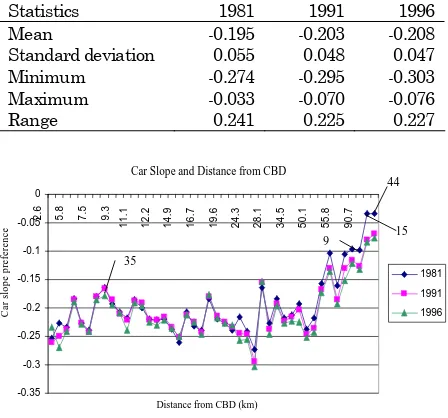
Table 1 is a summary of descriptive statistics of the slope for commuting preferences by car in Sydney over a 15-year period from 1981 to 1996. The absolute value of the mean slope preference by car increased by 0.013 over this period from 0.195 in 1981 to 0.208 in 1996.
Figure 2 shows the slope preferences by car for 44 LGAs in Sydney by increasing LGA distances from the CBD over a 15-year period from 1981 to 1996. The slope preferences by car for the inner and middle ring residents (within 20 km of the CBD) are relatively stable. In contrast, the outer ring residents, beyond 20 km from the CBD mainly experienced a significant increase.
Several LGAs show drastic changes of the slope preferences as shown in Figure 3. South Sydney (Zone 35) experienced the highest increase in the inner ring in absolute terms (about 0.015 per five years). Auburn (Zone 2) had the highest increase in the middle ring. Several extreme cases were found in the outer ring such as in Gosford (Zone 15), Camden (Zone 9), and Wyong (Zone 44).
The findings indicate that decentralization of employment towards the outer areas increased the behavioral preferences by car of residents in these outer areas towards longer trips, or a maximizing behavioral response. Therefore, future distribution of employment needs to be carefully located, because decentralization of employment is not associated with minimizing distance behavior for travel to work by car for outer ring residents.
Table 1. Summary of descriptive statistics of the slope
preferences by car in Sydney
Statistics 1981 1991 1996
Mean -0.195 -0.203 -0.208
Standard deviation 0.055 0.048 0.047
Minimum -0.274 -0.295 -0.303
Maximum -0.033 -0.070 -0.076
Range 0.241 0.225 0.227
Car Slope and Distance from CBD
-0.35
Distance from CBD (km)
C
Figure 2. Slope preference by car in Sydney by increasing
distance from the CBD
Figure 3. Change of slope preference by car in Sydney per
five years by increasing distance from the CBD
Analysis of Commuting Preferences by Bus
Table 2 summaries descriptive statistics of the slope preferences by bus in Sydney over a 15-year period from 1981 to 1996. The descriptive statistics reveal that the absolute value of the slope preferences by bus has increased from 0.150 in 1981 to 0.169 in 1996. This indicates that the behavioral preference of residents for commuting by bus has moved toward longer trips or distance maximizing trends.
By increasing LGA distances from the CBD, Figure 4 shows that the absolute value of the slope preferences by bus tend to decrease. This indicates that LGAs located further away from the CBD have preferences towards shorter trips to work by bus. Residents in the outer ring tend to use bus for local or short distance commuting trips only.
Table 2. Summary of descriptive statistics of the slope
preferences by bus in Sydney
Statistics 1981 1991 1996
Mean -0.150 -0.160 -0.169
Standard deviation 0.089 0.101 0.120
Minimum -0.292 -0.470 -0.676
Maximum -0.009 -0.025 -0.028
Range 0.283 0.445 0.648
Bus Slope and Distance from CBD
-0.7
Distance from CBD (km)
Sl
Figure 4. Slope preference by bus in Sydney by increasing
Figure 5 shows the average change of slope preference by bus per five years by increasing distance from the CBD. On average in the outer ring, the slope preference by bus has increased by about 0.091 per five years. On the other hand, residents in the inner ring tend to use bus for traveling to work for longer distance commuter trips. A substantial increase in the absolute value of the slope preferences by bus is experienced in the Sydney (Zone 38) (about 0.145 per five years from 0.240 in 1981 to 0.676 in 1996).
Figure 5. Change of slope preference by bus in Sydney per
five years by increasing distance from the CBD
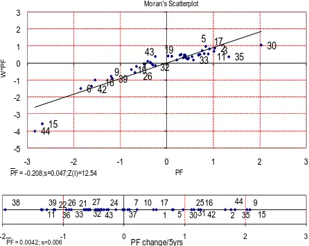
Spatial Analysis of the Commuting Preferences by Car
Figure 6 shows the Moran’s scatter-plot for the slope preferences by car in Sydney in 1996. To facilitate interpretation, the variables have been normalized with respect to the mean (PF) and standard deviation (s). The PF is used as a spatial variable
and analyzed using Moran’s I. The result indicates a
positive spatial autocorrelation where similar values
are found at neighboring locations with I = 0.562.
The Z-statistic, Z(I) = 11.729 (α = 0.05) shows that
the pattern deviates significantly from a random pattern where the zones interact with others with similar preference. Figure 6 shows that the zonal slope preferences by car in Sydney in 1996 are predominantly within one standard deviations of the mean. However, Parramatta (Zone 30) is found to have a value of the slope preference by car that is more than two standard deviations higher than the mean (on horizontal axis of Figure 6) despite the fact that it has a relatively high concentration of employment and is regarded as the second CBD in Sydney. On the other hand, Wyong (Zone 44) and Gosford (Zone 15) have values that are more than two standard deviations lower than the mean
(negative side of the horizontal axis). The relative isolation of Wyong and Gosford from the other LGAs has shaped residents preference for shorter travel and many find their jobs locally.
At the bottom part of Figure 6, a scatter-plot of the average change in the slope preference by car per five years is presented. It is shown that the LGAs in Sydney mainly experienced changes in the slope preferences by car with values within one standard deviation of the mean. However two extreme cases were identified. Although having a low slope preference by car (absolute), Gosford (Zone 15) and Camden (Zone 9) experienced an increase in the absolute value of the slope preference by car per five years and was over two standard deviations higher than the mean. Increasing numbers of job opportunities available in this LGA and surrounding LGAs over time as a result of decentralization, have changed the behavioral response of residents towards distance maximization, where an increasing number of people are employed in the other surrounding LGAs.
35
7 32
43
33 11 3
2 30
26 19
9 10
42
5
6
17
16 39
4415
-5 -4 -3 -2 -1 0 1 2 3
-3 -2 -1 0 1 2 3
PF
W*
P
F
_
PF = -0.208;s=0.047;Z(I)=12.54
Moran's Scatterplot
35
38 7
32 43 24 27
1 21
33
11 36 30 2
22 26
37
9 10
42 25 5 31
17 16
39 44
15
-2_ -1 0 1 2 3
PF = 0.0042; s=0.006 PF change/5yrs
Note: Numbers indicate zone number, PF = Preference Function
Figure 6. Moran’s scatter-plot for slope preferences by car
using O-D matrix
Figure 7 further shows Moran’s scatter-plot for the zonal slope preference by car considering destination-origin (D-O) matrix or demand side. Zones with minimization preferences (low value of slope preference) tend to attract trips from zones with similar preferences whilst zones with maximization preferences (high value of slope preference) tend to attract zones also with maximization preferences. The result of Moran’s
I (I = 0.710) indicates the existence of positive
spatial autocorrelation which is statistically
35
Moran's Scatterplot Car (D-O)
Note: Numbers indicate zone number, PF = Preference Function
Figure 7. Moran’s scatter-plot for slope preference by car
using D-O matrix
Spatial Analysis of the Commuting Preferences by Bus
Figure 8 shows the Moran’s scatter-plot for the distribution of zonal slope preferences by bus in Sydney in 1996. The variation of zonal slope preferences by bus is not very extreme as most of the slope preferences are within one standard deviation and only a few zones are beyond one standard deviation on either the minimization or the maximization side. However, one extreme case is identified where Sydney (Zone 38) has slope preferences beyond four standard deviations on the
maximization side. Moran’s statistic of I = 0.650,
indicates the existence of positive spatial autocorrelation. Further significance testing
with Z-statistic, Z(I) = 10.39 (α = 0.05) indicates
the significance of this positive spatial autocorrelation. The residents in the zones with high slope (preferences towards longer trips) tend to interact with zones having high values (absolute) of slope preferences. On the other hand, the residents in zones with low absolute slope preferences tend to travel to zones also with low absolute slope or zones with preferences towards distance minimization. Scatter-plot of the average change in the slope preferences by bus per five year shown at the bottom of Figure 8 indicates that the values are mainly within one standard deviation from the mean. Only one extreme case was identified where Sydney (Zone 38) experienced an increase in the slope preference by bus of over six standard deviations above the mean value. This indicates an increasing preference of residents in Sydney LGA to use bus for traveling to work for longer distances over time given already having a high absolute value.
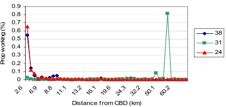
Figure 9 explains further that an extensive bus
service in the inner areas (within 11 km from the CBD), enable people living in the inner ring to travel longer by bus to reach their work place, in particular, to the CBD destination (for example in the figure,
Sydney (Zone 38) and Leichardt (Zone 24)). Residents living in Sydney tend to travel longer by bus to reach their work place given the high intensity of bus services in this LGA. People living in outer areas such as Penrith (Zone 31) tend to take the bus mainly for local and relatively short trips, whilst car dominates long distance trips. The proportion of workers using bus in the outer areas is much lower than that in the inner and middle areas because of the lack of reliable bus services. Low density and scattered jobs locations make it much more convenient for these outer ring residents to travel by car.
PF = -0.169;s=0.118;Z(I)=10.39
Moran's Scatterplot (Bus)
PF = 0.0064; s=0.023 PF change/5yrs
Note: Numbers indicate zone number, PF = Preference Function
Figure 8. Moran’s scatter-plot for slope preferences by bus
Proportion Working by Bus Vs Dis tance from CBD
0
Distance f rom CBD (km)
P
Figure 9. Proportion of residents working by bus by
increasing distance from the CBD
By considering the destination-origin (D-O) matrix, a positive spatial association is also experienced as shown in Moran’s scatter-plot (Figure 10). Zones with preference towards distance maximization tend to attract trips from zones which also show maximization preferences. On the other hand, zones with preference towards distance minimization tend to attract trips from zones with similar preferences. This positive spatial association is confirmed further
from Moran’s I statistic with I = 0.589 and Z(I) = 4.90
35 38 43
40 27 1
29
20 2133 11
3 30
12 34 22
41
37 42 5 6
31 17
15
-2 -1,5 -1 -0,5 0 0,5 1 1,5 2
-2 -1 0 1 2 3 4 5
PF
W*
P
F
_
PF = -0.169;s=0.118;Z(I)=4.90
Moran's Scatterplot Bus (D-O)
Figure 10. Moran’s scatter-plot for slope preferences by
bus using D-O matrix
Conclusions
The results of preference functions analyses indicated that the mean slope preference by car has increased over time showing an increasing preference of residents towards distance maximization for traveling to work by car. The slope preferences by car for the inner and middle ring residents are relatively stable over time whilst the outer ring residents (beyond 20 km from the CBD) experienced a dramatic increase. Similarly the commuting preference by bus is found to move towards distance maximization over time. By increasing distances from the CBD, the absolute values of slope preferences by bus tend to decrease. This shows that the outer ring residents tend to use bus for shorter distance trips (more than that of the inner and middle ring residents). For the zonal slope preferences by car, a significant positive spatial association was identified for both supply and demand sides. Zones with a preference towards long trips, on average, tend to travel to zones that also prefer longer trips. On the other hand, zones with a preference towards shorter trips, travel to zones that also have preference for shorter trips.
A significant positive spatial association is also identified for the slope preferences by bus for both O-D and O-D-O matrices. One extreme case is identified where Sydney LGA (Zone 38) has slope preferences beyond four standard deviations on the maximization side. Scatter-plot of the average change in the slope preferences by bus per five years further indicates that the Sydney LGA has an extreme value. The change in the slope preferences by bus in the Sydney LGA is over six standard deviations higher than the mean value. This indicates an increasing preference of residents in the Sydney LGA (CBD) to use bus for traveling to work for longer distances over time. It is clearly shown from these results that when increasing job opportunities are available in the surrounding zones, residents tend to travel longer to reach job opportunities available in the other zones, in particular, in the case of job-skill mismatch. Therefore,
it is not surprising that a dramatic increase in preference for longer trips has been experienced by outer ring residents in Sydney where job decentralization continues to occur over time.
References
1. WHO, Health Effects of Transport-Related Air
Pollution, World Health Organization, Copenhagen,
2005.
2. Newman, P. and Kenworthy, J., Sustainability
and Cities: Overcoming Automobile Dependence, Island Press, Washington, D.C., 1999.
3. Yang, J., Commuting Impacts of Spatial Decentralization: A Comparison of Atlanta and
Boston, Journal of Regional Analysis and Policy,
35(1), 2005, pp. 70-78.
4. Schwanen, T. and Mokhtarian, P.L., What
Affects Commute Mode Choice: Neighborhood Physical Structure or Preferences Toward
Neighborhoods? Journal of Transport Geography,
13, 2005, pp. 83-99.
5. Hamilton, B.A., Study of Successful Congestion
Management Approaches and the Role of Charging, Taxes, Levies and Infrastructure and Service
Pricing in Travel Demand Management, Council
of Australian Governments, 2006.
6. Holmgren, J., Jansson, J.O., and Ljungberg, A.,
Public Transport in Towns–Inevitably on the
Decline? Research in Transportation Economics,
23, 2008, pp. 65–74.
7. Joewono, T.B. and Kubota, H., Exploring Public Perception of Paratransit Service using Binomial
Logistic Regression, Civil Engineering Dimension,
9(1), 2007, pp. 1-8.
8. Mulley, C., and Nelson, D., Flexible Transport Services: A New Market Opportunity for Public
Transport, Research in Transportation Economics,
25, 2009, pp. 39-45.
9. Pooley, C.G., and Turnbull, J., Modal Choice and Modal Change: The Journey to Work in Britain
since 1890, Journal of Transport Geography, 8,
2000, pp. 11-24.
10. Montis, A.D., Chessa, A., Campagna, M., Caschili, S., and Deplano, G., Modeling Commuting Systems through a Complex Network Analysis: A Study of the Italian Islands of Sardinia and Sicily,
Journal of Transport and Land Use, 3(4), 2010,
pp. 39-55.
Data, Networks and Spatial Economics, 7(4), 2007, pp. 315–331.
12.Black, J., Paez, A. and Suthanaya, P., Sustainable
Urban Transportation: Performance Indicators
and Some Analytical Approaches, American
Society of Civil Engineers. Journal of Urban Planning and Development, Special Issue: Advances in Urban Planning Methodologies I: Recent
Advances, 128(4), 2002, pp. 184-209.
13.Ruiter, E.R., Improvement in Understanding,
Calibrating and Applying the Opportunity Model,
Highway Research Record, 165, 1969, pp. 1-21.
14. Stouffer, S.A., Intervening Opportunities: A Theory
Relating Mobility and Distance. American
Sociological Review, 5, 1940, pp. 347-356.
15. Moran, P., The Interpretation of Statistical Maps,
Journal of the Royal Statistical Society B, 10,
1948, pp. 243-251.
16.Cliff, A.D. and Ord, J.K., The Problem of Spatial
Autocorrelation, Scott, A.J. (ed.), Studies in
Regional Science, Pion, London, 1969.
17.Anselin, L., Local Indicators of Spatial Association–