ANSWERING GEOSPARQL QUERIES OVER RELATIONAL DATA
K. Beretaa, G. Xiaob∗, M. Koubarakisa
aDepartment of Informatics and Telecommunications, University of Athens, Greece - (konstantina.bereta,koubarak)@di.uoa.gr b
Free University of Bozen-Bolzano, Italy- [email protected]
Commission IV, WG IV/4
KEY WORDS:GeoSPARQL, RDF, Ontology-based Data Access
ABSTRACT:
In this paper we present the system Ontop-spatial that is able to answer GeoSPARQL queries on top of geospatial relational databases, performing on-the-fly GeoSPARQL-to-SQL translation using ontologies and mappings. GeoSPARQL is a geospatial extension of the query language SPARQL standardized by OGC for querying geospatial RDF data. Our approach goes beyond relational databases and covers all data that can have a relational structure even at the logical level. Our purpose is to enable GeoSPARQL querying on-the-fly integrating multiple geospatial sources, without converting and materializing original data as RDF and then storing them in a triple store. This approach is more suitable in the cases where original datasets are stored in large relational databases (or generally in files with relational structure) and/or get frequently updated.
1. INTRODUCTION
This paper describes the system Ontop-spatial (Bereta and Koubarakis, 2016), which provides semantic data integration for geospatial data, creating virtual geospatial RDF graphs on top of geospatial databases and enabling on-the-fly GeoSPARQL-to-SQL translation.
In the recent years, there is an emerging interest from researchers of various domains (e.g., earth scientists, geologists, cartogra-phers, civil engineers) that are involved in the processing of geospatial data, to publish them as RDF data to increase its value by combining it with other open data. As a result, the Web of data is populated with a rapidly increasing amount of geospatial data bringing challenges that have been addressed by the Seman-tic Web community proposing data models, query languages and applications for the representation, modeling and visualization of linked geospatial data.
These efforts have been highlighted by the establishment of the Open Geospatial Consortium (OGC) standard GeoSPARQL, a geospatial extension of RDF and SPARQL (Open Geospatial Consortium, 2012). Other extensions of RDF and SPARQL were also proposed, such as the framework of stRDF and stSPARQL which extends RDF and SPARQL with both space and time fea-tures (Kyzirakos et al., 2010, Bereta et al., 2013). These stan-dards of geospatial support have also been implemented in sev-eral RDF stores, such as Parliament1, uSeekM2, Virtuoso3, Star-dog4 and Strabon5 (Kyzirakos et al., 2012). These technologies enabled geospatial data practitioners to (i) convert their data (usu-ally relational like) into interoperable data formats such as RDF, (ii) store the data in RDF format into geospatial RDF stores to-gether with other geospatial data, and (iii) express rich geospatial queries combining multiple datasets, as for example the query Retrieve all flooded areas in Europe that overlap with water bod-ies (according to CORINE), and points of interest (from
Open-∗Corresponding author
1
http://parliament.semwebcentral.org
2
https://www.w3.org/2001/sw/wiki/USeekM
3
https://virtuoso.openlinksw.com
4
http://www.stardog.com/
5
http://strabon.di.uoa.gr
StreetMap) near them. This query retrieves information about floods, combined with two other open geospatial datasets, namely the RDF version CORINE Land Cover dataset6, and the RDF ver-sion of OpenStreetMap data7.
In practice geospatial data are often originally stored in geospa-tial DBMSs (e.g. PostGIS and Oracle). Especially in the cases when these databases get frequently updated, some users are dis-couraged to convert the data into RDF and store it to triple stores every time new updates arrive. Thus, in these cases the value of this data cannot be interlinked with other linked open data to increase its value.
The Semantic Web community addressed this issue by develop-ing Ontology-Based Data Access (OBDA) techniques and sys-tems that offer on-the-fly SPARQL-to-SQL translation based on ontologies and mappings, such as Ontop8and Morph-RDB9. Us-ing the OBDA approach, one can create semantic RDF graphs on top of relational data using ontologies and mappings. Map-ping is a way to encode how relational data can be translated into RDF terms. The standard language for encoding mappings is the R2RML mapping language10. In OBDA, one avoids materializa-tion of the relamaterializa-tional data into RDF; SPARQL queries are trans-lated into SQL on-the-fly and are evaluated by the underlying DBMS.
However, existing OBDA systems did not provide support for geospatial data until the creation of Ontop-spatial. Ontop-spatial, the geospatial extension of the OBDA system Ontop, is able to connect to geospatial databases and create geospatial RDF graphs on top of them using ontologies (that are extensions of the GeoSPARQL ontology) and mappings. This virtual approach avoids the need of materialization and facilitates data integra-tion, as it enables users to pose the same GeoSPARQL queries they would pose over the materialized RDF data. GeoSPARQL queries are translated by Ontop-spatial on-the-fly into the respec-tive SQL queries and are evaluated in the geospatial DBMS.
Cur-6
https://datahub.io/dataset/corine-land-cover
7
http://linkedgeodata.org/
8
http://ontop.inf.unibz.it
9
https://github.com/oeg-upm/morph-rdb
10
https://www.w3.org/TR/r2rml/
The International Archives of the Photogrammetry, Remote Sensing and Spatial Information Sciences, Volume XLII-4/W2, 2017 FOSS4G-Europe 2017 – Academic Track, 18–22 July 2017, Marne La Vallée, France
This contribution has been peer-reviewed.
rently, PostGIS, Spatialite and Oracle Spatial are supported as back-end.
We have evaluated Ontop-spatial by extending the benchmark Geographica11, which was initially designed to evaluate the per-formance of geospatial RDF stores, with support for OBDA systems. We compared Ontop-spatial with the state-of-the-art geospatial RDF store Strabon. The results showed that in Ontop-spatial generally achieves significantly better performance than Strabon.
This paper is structured as follows. First, we present related back-ground information in Section 2. and in Section 3. we present re-lated work in this area. In Section 4. we describe in detail the im-plementation of our approach in the system Ontop-spatial and in Section 5. we measure the peformance of our implementation in comparison to the state-of-the-art. Finally, Section 6. concludes the paper and Section 7. presents future work.
2. BACKGROUND
This section presents background information in the area of the Semantic Web and the technologies and frameworks that form the context in which our work has been developed.
2.1 RDF and SPARQL
We describe below fundamental concepts of the data model RDF and the query language SPARQL, as defined in (P´erez et al., 2009).
Definition 1. RDF triple. LetI, BandLbe pairwise disjoint infinite sets.Irepresents the st of IRIs,Bthe set of blank nodes, andLrepresents the set of Literals. An RDFtripleis a tuple of the form(s, p, o)∈(I∪B)×I×(I∪B∪L), wheresis the subject,pis the predicate, andois the object.
Definition 2. An RDF graph is a set of RDF triples.
Definition 3. A SPARQL query is a tuple of the form(V, P, G), whereP is a SPARQL algebra expression,V is the set of vari-ables that occur inP, andGis an RDF graph.
Definition 4. Atriple patternis a tuple of the form(I∪L∪V)×
(I∪V)×(I∪L∪V).
Definition 5. A graph pattern is defined recursively as one of the following:
• a triple pattern
• an expression of the formP1OPP2, where OP is one of the SPARQL algebraic operators:AND,UNION,OPT.
• an expression of the formPFILTERR, wherePis a graph pattern andRis a SPARQL built-in condition. A SPARQL built-in condition is a boolean expression that is constructed using elements of the set V ∪IL and constants, logical connectives(¬,W,V), equality (=) and inequality symbols
(≥,≤, <, >), unary predicates (bound, isBlank, isIRI), and other features.
11
http://geographica.di.uoa.gr
2.2 stRDF and stSPARQL
An example of an RDF triple is provided below.
PREFIX ex : <http://example.com>
PREFIX rdf: <https://www.w3.org/TR/rdf-schema/>
ex:id434 rdf:type ex:school .
The triple described above denotes that the entity identified with the URI ex:id434 is a school.
Since the framework of RDF and SPARQL does not contain sup-port for the representation and querying of geometries, as soon as the first geospatial datasets appeared in the web of data as RDF, the need for representing geospatial features properly emerged. Several extensions of the data model RDF and the query lan-guage stSPARQL were proposed in literature. The data model stRDF and the query language stSPARQL are extensions of RDF and SPARQL 1.1 respectively, developed for the representation and querying of spatial (Kyzirakos et al., 2012) and temporal data (i.e., the valid time of triples (Bereta et al., 2013)). More specifically, the data model stRDF proposes the representation of geometries as literals of the datatypes Well-known-text (WKT) and GML, that are OGC standards. The temporal dimension of the data model stRDF introduces also the perioddatatype, allowing intervals to be represented as literals of the datatype
strdf:period. Similarly, the query language stSPARQL allows
spatial operations on geometries as well as temporal operations on instants and periods. The framework of stRDF and stSPARQL also introduces the valid time dimension: a fourth element can be added to a triple to represent thevalid timeof a triple, i.e., the time when the fact represented by the triple is valid. The valid time of a triple can be represented either by a timestamp (i.e.,
anxsd:datetimeliteral) or a period (i.e., anstrdf:period
literal). By this way, the framework of stRDF and stSPARQL is suitable for the representation and querying of geospatial data that changes over time.
2.3 GeoSPARQL
Figure 1. GeoSPARQL components
Figure 2. GeoSPARQL ontology
Core component. This component defines high level RDF-S/OWL classes for spatial objects. The GeoSPARQL class hi-erarchy can be seen in Figure 2 and the respective ontology can be accessed athttp://www.opengis.net/ont/geosparql.
Topology vocabulary extension. This component defines RDF properties for asserting and querying topological relations be-tween spatial objects and covers different families of topological relations, such as Simple Features Access, RCC8, and Egenhofer.
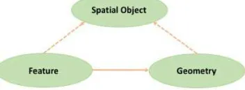
Geometry extension. The Geometry extension component de-fines the literal representation of geometries by introducing new datatypes that correspond to the OGC standards WKT and GML
respectively. In order to connect features with their geome-tries and the serializations of these geomegeome-tries, the properties geo:hasGeometry,geo:hasSerialization are also defined in this component of GeoSPARQL. For example we provide the follow-ing RDF graph:
ex:id434 rdf:type ex:school . ex:id434 geo:hasGeometry ex:geo1 .
ex:geo1 geo:asWKT "POINT(23.7,37.9)"^^geo:wktLiteral .
The set of triples described above denote that ex:id434 is a school that has a geometry and the WKT representation of this geometry
isPOINT(23.7,37.9).
Geometry Topology extension. This component defines a set of functions that can be used in queries to evaluate topological operations between geometries.
RDFS entailment extension. This extension basically includes RDF and RDFS reasoning support. By this way, GeoSPARQL queries that are posed against GeoSPARQL endpoints that im-plement this component of GeoSPARQL will not only consider the triples that are explicitly included in the knowledge base, but
only the ones that can be derived from the knowledge base and the ontology.
Query rewrite extension. This component of GeoSPARQL de-fines a set of transformation rules that convert geospatial qualita-tive queries into quantitaqualita-tive ones, when explict qualitaqualita-tive infor-mation is not available in the knowledge base. For example, let us consider the qualitative GeoSPARQL query described in Figure 3.
SELECT ? x WHERE { ? x geo : s f O v e r l a p s ? y
Figure 3. Example of a spatial qualitative query
The query described above retrieves features that ovelap with each other. However, results will be returned only if the respec-tive qualitarespec-tive information exists in the knowledge base, for ex-ample a triple similar to the following:
ex:geo1 sf:Overlaps ex:geo2 .
The triple provided above denotes that two features identified with the URIsex:geo1and ex:geo2overlap with each other. But in the case when no such information exists in the knowl-edge base, but aternatively the actual geometry representations of the respective features are available, then the query provided above could be transformed into the query described in Figure 4.
SELECT ? x WHERE { ? x geo : asWKT ? geo1 . ? y geo : asWKT ? geo2 .
FILTER ( geof : s f O v e r l a p s (? geo1 , ? geo2 ))}
Figure 4. Example of a spatial quantitative query
2.4 Linked Open Data
The framework of Linked Data is a paradigm which brings data as first class citizens of the Web and it involves a set of technolo-gies and methodolotechnolo-gies, described in (Heath and Bizer, 2011) so that following this paradigm, data can be published and con-sumed easily both by machines and humans, in compliance to well-established open standards.
As described in (Heath and Bizer, 2011), the Linked Data paradigm in a nutshell includes the following principles:
• Data should be published as RDF.
• Resources should be represented by dereferencable URIs, so that they can be looked up.
• Data should be available via SPARQL endpoints so that they can be queried using SPARQL.
• Data should be interlinked: Links that connect resources be-tween the same or different datasets that are published as Linked Open Data should be discovered, materialized and published as well. By this way, the value of the original data is increased by the correlation to other information that is available on the Web.
The International Archives of the Photogrammetry, Remote Sensing and Spatial Information Sciences, Volume XLII-4/W2, 2017 FOSS4G-Europe 2017 – Academic Track, 18–22 July 2017, Marne La Vallée, France
This contribution has been peer-reviewed.
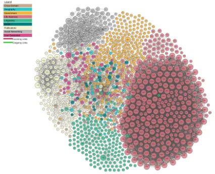
Figure 5. Linking Open Data cloud diagram 2017, by A. Abele, J. P. McCrae, P. Buitelaar, A. Jentzsch and R. Cyganiak
The EU project LOD212 focused on developing methodologies and tools to define and implement the different phases of extract-ing, publishing and querying of data as linked open data.
Figure 5 shows the Linked Open Data cloud13. In this figure, datasets that are currently available as Linked Open Data are rep-resented as circles whose size is analogous to the size of the re-spective dataset. The datasets are grouped in different categories according to the domain they belong to and the arrows that exist between the datasets represent the links that connect their enti-ties. Geospatial datasets that are available as Linked Open Data have blue colour.
The EU research projects LEO14 developed tools and method-ologies for publishing Earth Observation data as linked data, ex-tending the work done by the project LOD2. In the context of this work, the lifecycle of Linked earth observation data was de-fined and implemented, as described in detail in (Koubarakis et al., 2016) and shown in Figure 6 .
Interlinking!
Publishing!
Storage/Querying!
Transformation! into RDF!
Semantic! Annotation! Knowledge Discovery!
and Data Mining! Content Extraction!
Data Cleaning! Search/Browse/! Explore/Visualize!
Ingestion!
Processing!
Archiving! Cataloguing!
Figure 6. The lifecycle of Linked Earth Observation Data
2.5 Ontology-based Data Access (OBDA)
Although the value of the linked data paradigm has been widely recognized by the scientific and industrial communities, its adop-tion by users is sometimes a challenging task. Especially in the
12
http://lod2.eu/Welcome.html
13
http://lod-cloud.net/
14
http://www.linkedeodata.eu/
as Linked data and increase its value by correlating it with other datasets.
Ontology-based data access (OBDA) refers to technologies that aim at accessing the data using ontologies but without material-izing it as RDF triples, allowing the on-the-fly creation of vir-tualRDF graphs instead. This is achieved usingmappings as first class citizens. Mappings encode how relational data cor-respond to RDF terms. The standard language for encoding this information is the W3C standard R2RML15. Parallel -and in most cases prior- to the development of R2RML, most OBDA systems supported their own mapping languages. For example, the sys-tem Ontop supports also its native OBDAlanguage apart from R2RML. The mappings that will be given as examples in the rest of this paper will follow this native mapping language of Ontop for the convinience of the reader, as it is more compact and easily readable.
3. RELATED WORK
In this section we briefly highlight related systems for querying linked geospatial data.
3.1 Geospatial RDF stores
There is wide variety of geospatial triple stores that imple-ment a big subset of GeoSPARQL specification, such as Stra-bon (Kyzirakos et al., 2010), that also implements stRDF and stSPARQL, Parliament16, uSeekM17, and Virtuoso18that supports some geospatial features but not the GeoSPARQL specification. In a recent study described in (Garbis et al., 2013), it is shown that Strabon is the most efficient in terms of performance and the most rich in functionalities geospatial RDF store that supports GeoSPARQL. Strabon is distributed as free and open source soft-ware.19
3.2 OBDA systems
In the area of Ontology-based data access, there are a few OBDA systems that offer on-the-fly SPARQL-to-SQL translation on top of relational databases, such as Ontop (Rodriguez-Muro and Rezk, 2015), Ultrawrap (Sequeda and Miranker, 2013), D2RQ20 and Morph (Priyatna et al., 2014). Although these systems have been available for some time now, there was no geospatial support in them until the creation of Ontop-spatial (Bereta and Koubarakis, 2016), the geospatial extension of the open source system Ontop that is also presented in this paper. Recently, GeoSPARQL OBDA support was added in Oracle Spatial and Graph, which is now part of Oracle 12c Release 2.
4. IMPLEMENTATION OF ONTOP-SPATIAL
In this section we present our geospatially-enhanced OBDA ap-proach and its implementation in the system Ontop-spatial21as a geospatial extension of the open source system Ontop.
15
https://www.w3.org/TR/r2rml/
16
http://parliament.semwebcentral.org
17
https://www.w3.org/2001/sw/wiki/USeekM
18
https://virtuoso.openlinksw.com
19
http://strabon.di.uoa.gr
20
http://d2rq.org/
4.1 Geospatial Mappings
Mappings play a crucial role in the OBDA paradigm. In the fol-lowing, we provide an example. Figure 7 shows a PostGIS ta-ble with the following columns: id,srid andstrdgeo. The column with namestrdfgeostores geometries in Well-known-binary (WKB) format, and the columnsridstores the code of the Coordinate Reference System (CRS) in which these geometries are expressed. In this case, all geometries are represented using the World Geodetic System 1984 (WGS84) that corresponds to the CRS code 4326.
Figure 7. Table schema
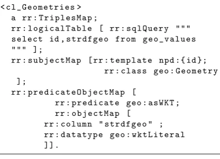
Now we want to represent the relational data of the table depicted in Figure 7 as virtual triples. Figure 8 shows how this can be encoded using the language R2RML and Figure 9 shows the re-spective representation in the Ontop native OBDA language. Ac-cording to the mapping shown in Figure 8, virtual triples are cre-ated that represent the serialization of geometries as literals of the datatypegeosparql:wktLiteral. It is signified that these virtual triples are not created beforehand or materialized. When a GeoSPARQL query arrives that involves these triples, the re-spective SQL query takes part in the resulting SQL query that is produced after the GeoSPARQL-to-SQL translation that is de-scribed in more detail in 4.2. Notably, although the source SQL query in the mappings retrieves the geometry column to populate the respective WKT literals as-is, i.e., in binary format, the result-ing virtual triples are in WKT format. This translation is carried out internally by the system.
< cl_Geometries > a rr : T r i p l e s M a p ;
rr : l o g i c a l T a b l e [ rr : s q l Q u e r y """ select id , s t r d f g e o from g e o _ v a l u e s """ ];
rr : s u b j e c t M a p [ rr : t e m p l a t e npd :{ id }; rr : class geo : G e o m e t r y ];
rr : p r e d i c a t e O b j e c t M a p [
rr : p r e d i c a t e geo : asWKT ; rr : o b j e c t M a p [
rr : column " s t r d f g e o " ; rr : d a t a t y p e geo : w k t L i t e r a l ]].
Figure 8. R2RML mappings
The mappings illustrated in Figure 9 encode similar information, but the source SQL query slightly deviates from the respective SQL query of the R2RML mappings in Figure 8, as it also con-tains the PostGIS functionST Transform. This function trans-forms the geometries stored in the table shown in Figure 7 to the Coordinate Reference System wth EPSG code 3035 on-the-fly, so the WKT representation of thetransformedgeometries will be the object of the virtual triples. This example demonstrates the
flexibility that is offered by the use of mappings and the OBDA paradigm in general; relational data can be pre-processed on-the-fly before being transformed as virtual triples. Following the tra-ditional approach, an extra pre-processing step would be added for the manipulation of the data and the tranformed data would need to be materialized. Following the approach that we propose, the original data remain intact and each time we want to change the kind of pre-processing that needs to be performed we simply change the mappings instead of changing the actual data.
[ M a p p i n g D e c l a r a t i o n ]
[[ m a p p i n g I d mapping - 7 6 7 3 5 1 7 7 9 target npd :{ id } a geo : G e o m e t r y ;
geo : asWKT { geo }^^ geo : w k t L i t e r a l source SELECT id ,
S T _ T r a n s f o r m ( strdfgeo , 3035) as geo FROM g e o _ v a l u e s ]]
Figure 9. OBDA mappings
4.2 GeoSPARQL-to-SQL translation
We have developed a GeoSPARQL-to-SQL approach by extend-ing a state-of-the-art SPARQL-to-SQL approach described in (Rodriguez-Muro and Rezk, 2015). In a nutshell, the SPARQL-to-SQL approach that is presented in (Rodriguez-Muro and Rezk, 2015) comprises the following major steps:
• A SPARQL query arrives and it is translated into a Datalog program
• After several optimizations and simplifications taking place, taking into account the mappings, and the schema and some characteristics of tables that are involved in the mappings (e.g., constraints) and the the final Datalog program is pro-duced.
• The Datalog program is translated into an SQL query that is evaluated by the underlying DBMS that serves as back-end.
• After the evaluation of the SQL in the DBMS, the results are returned as RDF terms, according the ontology and the mappings that have been given as input.
In order to support GeoSPARQL, we have extended the approach described above (and in more detail in (Rodriguez-Muro and Rezk, 2015)) as follows:
• A GeoSPARQL query arrives and gets translated into Data-log.
• If the GeoSPARQL query contains functions in the filter clause, each function is represented in the Datalog program by the respective geospatial predicate that we have intro-duced. If the GeoSPARQL query contains a GeoSPARQL predicate instead of a function, then the Datalog program contains the same geospatial predicate. By this way, both quantitative and qualitativegeospatial queries are treated uniformly. Quantitative geospatial queries are those that in-clude operations on geometries (e.g., geometries ovelapping each other). Qualitative geospatial qualitative geospatial queries is those who express qualitative geospatial relations between features, for which the geometries may or may not be known (e.g., Rivers that overlap with lakes). This is how
thequery rewritecomponent of GeoSPARQL is
imple-mented.
The International Archives of the Photogrammetry, Remote Sensing and Spatial Information Sciences, Volume XLII-4/W2, 2017 FOSS4G-Europe 2017 – Academic Track, 18–22 July 2017, Marne La Vallée, France
This contribution has been peer-reviewed.
• In the Datalog-to-SQL translation phase, the geospatial predicates that are included in the datalog program are trans-lated into the respective geospatial operators that are sup-ported by the underlying DBMS.
The GeoSPARQL-to-SQL translation that we described above is illustrated in figure 1 it it is also described in more detail in (Bereta and Koubarakis, 2016).
Our approach is implemented as a geospatial extension of the sys-tem Ontop, named Ontop-spatial22. It is available as free and open-source software, under GPL Apache License.
4.3 Beyond GeoSPARQL
Raster data support.
None of the geospatial extensions of the framework of RDF and SPARQL, such as stRDF and stSPARQL and GeoSPARQL have considered support for raster data. The main challenge that lies behind this is twofold: First, a raster file is associated with a ge-ometry only as a whole. It is not straight-forward to associate separate raster cells to a geometry, they have to be vector-ized first (i.e., translated into polygons). Second, every raster cell is associated with one or more values. In order to convert all infor-mation contained in a raster file into RDF, then multiple triples should describe a raster cell, producing a large amount of triples for a whole raster file. However, not all of this information is needed. In most of the use cases, only the information that de-rives from a raster file and qualifies certain criteria (e.g., value constraints) is all that is needed to be converted into RDF. This means that the raster file needs to be processed and then the re-sults of this processing are useful as RDF, while any other infor-mation is redundant. These challenges have discouraged the sci-entific community from converting and materializing raster data to RDF.
In the work described in this paper, we address these challenges by following the OBDA paradigm:
• Ontop-spatial can connect to a geospatial relational database with a raster adapter.
• The raster datatype is internally handled in the same way as its vector counterpart (e.g., the Geometry datatype).
• The following GeoSPARQL operators are overloaded for supporting the respective operations having raster data as arguments in addition to vector data: ST Contains,
ST Covers, ST Within, ST Overlaps, ST Intersects,
ST Touches.
• PostGIS operators can be added in the mappings in order to process the raster data and create virtual geospatial RDF views above them. For example, certain operators can be used in the SQL query of a mapping in order to refine the results, refining the information from the original raster file that will be virtually translated into RDF.
4.4 Beyond Relational databases
Even when data is not originally stored into relational geospatial databases, but is available in a format that can be easily imported into one (e.g., Shapefiles, GeoTIFF, etc.), exploiting the adapters
22
https://github.com/ConstantB/ontop-spatial
that many geospatial databases have implemented for widely-used geospatial file formats, our approach can still be widely-used. In this direction, we have extended our approach by supporting data sources without materializing them in relational tables. In this re-spect, Ontop-spatial now provides support for the system Madis23 (Chronis et al., 2016), an extensible relational database system built on top of an SQLite wrapper named APSW24. Madis sup-ports a query language that extends SQL with operators and pro-vides a Python interface so that users can easily implement user-defined functions (UDFs). An example is provided below.
Listing 1. MadIS query
select aa as id , onoma as name ,
" POINT ( " || long || " " || lat || " ) " as geo from ( file ’ http :// bit . ly /2 q8JiR6 ’ header : t )
In the query provided above, a csv dataset is retrieved from the Web using the file operator of Madis inside a SQL-like query. In the select clause of the query the WKT format of the geome-tries is constructed on-the-fly, using the longitude and latitude columns of the csv file. The ability of processing arbitrary file formats using extended SQL syntax offered by MadIS and its in-tegration to Ontop-spatial enables users to create mappings on top of datasets that are not relational and query the data as RDF us-ing (Geo)SPARQL. For example, a mappus-ing created for the data sources described above is given:
mappingId public_schools_gr
target :schools/{id} a :school; :hasName {name} ; geosparql:asWKT {geo} . source select aa as id, onoma as name,
"POINT(" ||long || " "||lat|| ")" as geo from (file’http://bit.ly/2q8JiR6’ header:t) limit 3
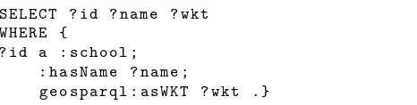
The mapping provided above encodes how the results returned by the MadQL query in the previous example can be mapped in RDF terms. The WKT representation of the geometries returned by the MadQL is used to create virtual triples that describe the ge-ometry extent of features. Using the approach that we described in Section 4.2 and in (Bereta and Koubarakis, 2016), one would have to download the .csv file first and then import it to a database and create mappings similar to the one provided above in order to use Ontop-spatial and pose GeoSPARQL queries against this dataset, such as the query described in FIgure 10, which, retrieves the names nad locations of schools.
Using MadIS as a back-end of Ontop-spatial, it is not necessary to download the file and import its contents into a materialized SQL table; When a GeoSPARQL query that involves this dataset arrives, the data will be fetched, made relational, evaluated and then returned as RDF on-the-fly, without being materialized in any intermediate level.
This gives the whole architecture a dynamic nature; Even if the data source is constantly updated, queries will retrieve the current version each time automatically.
5. EVALUATION
This section present the set up and the results of the experimental evaluation that we conducted in order to measure the performance of the implementation which we presented in Section 4.
In order to evaluate our system, we used a variation of the bench-mark Geographica(Garbis et al., 2013). Since Geographica was
23
https://github.com/madgik/madis
24
SELECT ? id ? name ? wkt WHERE {
? id a : school ; : hasName ? name ;
g e o s p a r q l : asWKT ? wkt .}
Figure 10. GeoSPARQL query
designed to evaluate the most recent advances in the area of geospatial RDF stores, and since there is no benchmark that spe-cializes in geospatial OBDA systems, we extended Geographica in the following two directions: (i) we added more datasets with more and more complicated (in terms of number of points per ge-ometry) geometries, and (ii) we extended the software framework of Geographica so that it also supports the evaluation of OBDA systems.
5.1 Datasets
Our workload comprises the following datasets:
• The Corine Land Cover dataset (CLC). This dataset is pro-vided by the European Environmental Agency25. We down-loaded only the data about Greece. The size of this dataset is 283 MB, it contains 44834 geometries, and each geometries contains about 187 points on average.
• The “Hotspots” dataset, i.e., a dataset about wildfires of Greece that was provided to us by the National Observatory of Athens. The size of this dataset is 35 MB and it contains 37048 geometries consisting of five points each.
• The Global Administrative Geography (GAG) dataset26. This dataset contains the boundaries (i.e., geometries) of all administrative divisions. We used only the respective infor-mation for Greece which is up to 24 MB in size, containing 326 geometries having about 3020 points each.
• Seven OpenStreetMap (OSM) datasets that are available as Shapefiles, one for each of the following categories: Build-ings, land use, places, points, railways, roads and water-ways. The total size of all seven datasets is about 350 MB and the total number of geometries contained in it is 810365. Some of these datasets contain only points (e.g., buildings, places, points), while others contain a little (e.g., railways with about 13 points per geometry) to more (e.g., waterways with about 40 points per geometry) complicated geometries.
All datasets provided above are available in Shapefile format. We imported all shapefiles into a PostGIS database and we connected this database with Ontop-spatial, after we created the respective ontology and mappings.
We decided to evaluate our geospatially-enhanced OBDA ap-proach to the traditional apap-proach, i.e., conversion of all data into RDF, importing the resulting RDF datasets to a geospatial triple store and then posing GeoSPARQL queries. We compared the execution time of GeoSPARQL queries in both Ontop-spatial and Strabon, which is the state-of-the-art geospatial RDF store, according to (Garbis et al., 2013). To be able to do so, we materi-alized thevirtualtriples that result from Ontop-spatial and stored them in Strabon, so that the two systems contain exactly the same
25
https://www.eea.europa.eu/data-and-maps/data/ clc-2006-vector-4
26
http://www.gadm.org/
information. The fact that both Strabon and Ontop-spatial are able to use PostGIS as back-end DBMS is convenient for our comparison.
5.2 Evaluation results
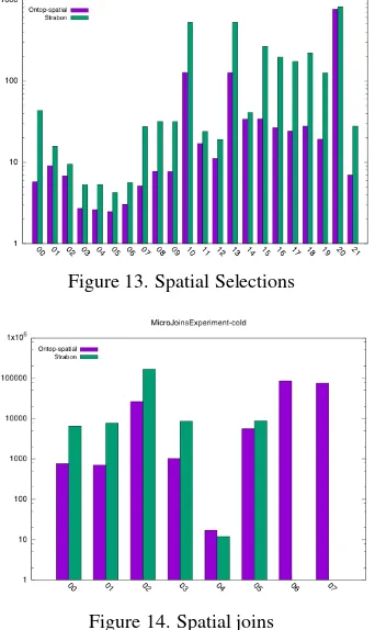
We executed a set of spatial selection queries and a set of spa-tial join queries and we measured the execution times in Ontop-spatial and Strabon,. In both cases the queries are executed in cold cache, as we clear the cache before each execution. Figure 11 shows an example of a spatial selection query which was in-cluded in the benchmark. Using this query we retrieve features whose geometry overlaps with a geometry which we provide as a constant. We created variations of this query testing different spa-tial operators (e.g.,sfContainsinstead ofsfOverlaps), adding more triple patterns, and different geometries as constants (i.g., points, lines, polygons). For example, we used both large and small polygons to produce qeuries of low and high selectivity re-spectively. An example of a spatial join query can be seen in Figure 12. Using this query we retrieve features with overlapping geometries. Notably, in spatial joins both arguments of the spatial filter functions are variables.
SELECT ? s1 ? o1 where { ? s1 lgd : asWKT ? o1 .
FILTER ( geo : s f O v e r l a p s ( C O N S T A N T _ G E O M ,? o1 ))}
Figure 11. Example of a spatial selection query
SELECT ? s1 ? o1 where { ? s1 lgd : asWKT ? o1 . ? s2 lgd : asWKT ? o2 . FILTER ( geo : s f O v e r l a p s (? o1 , ? o2 ))}
Figure 12. Example of a spatial join query
The results of the evaluation of the spatial selections and spatial joins can be seen in Figures 13 and Figure 14 respectively. The results show that Ontop-spatial outperformes Strabon, often by orders of magnitude. In Spatial joins 6 and 7 shown in Figure 14, Strabon times out after 40 minutes.
Ontop-spatial achieves better performance than Strabon mainly because the schema of the database is more natural, i.e., it is constructed by importing Shapefiles and each Shapefile corre-sponds to a table in the database. On the other hand, the PostGIS database in the back-end of Strabon stores triples, and this means that some more information about the triples (e.g., the vocabu-lary) is stored in the database. As a result, the database of Stra-bon is double the size of the database of Ontop-spatial. Moreover, the database that is produced by Strabon follows the star schema, i.e., each distinct predicate corresponds to a different database table and each kind of RDF datatypes are stored in dedicated ta-bles. So, all geometries of the knowledge base that is stored in Strabon are stored in a separate table with a geometry column, and an R-Tree is constructed on that column. On the other hand, in Ontop-spatial, there is one table per data source having a ge-ometry column and an R-Tree is constructed for every table with geometies based on that column. As a result, geometries are par-titioned in different tables/indices in the case of Ontop-spatial and in the case of spatial queries only the tables that are involved take part in the evaluation.
6. CONCLUSIONS
In this paper we presented an apprach for creating semantic vir-tual geospatial RDF graphs on top of geospatial data with rela-tional structure enhancing the OBDA paradigm with geospatial The International Archives of the Photogrammetry, Remote Sensing and Spatial Information Sciences, Volume XLII-4/W2, 2017
FOSS4G-Europe 2017 – Academic Track, 18–22 July 2017, Marne La Vallée, France
This contribution has been peer-reviewed.
Figure 13. Spatial Selections
Figure 14. Spatial joins
features, enabling users to perform GeoSPARQL queries on top of geospatial relational databases. The framework that we pro-pose can also be applied beyond geospatial databases, to data that can be logically viewed as relational (e.g., CSV files), and we also go beyond the OGC standard GeoSPARQL by supporting raster data as well.
7. FUTURE WORK
As for the future, we want to support GeoSPARQL over more non-relational data sources, e.g. GeoJSON documents stored in MongoDB27. We plan to investigate techniques for parallel geospatial query processing and extend our framework to en-able distributed GeoSPARQL query processing. We also plan to develop further optimization approaches, particularly in the cases where data is not natively stored in geospatial relational databases, but it is available in tabular format on the Web.
ACKNOWLEDGEMENTS
This work has been partially funded by the EU FP7 project OP-TIQUE (318338), the EU project Copernicus App Lab (730124), and the UNIBZ RTD project OBDAM (IN2045).
REFERENCES
Bereta, K. and Koubarakis, M., 2016. Ontop of geospatial databases. In: The Semantic Web - ISWC 2016 - 15th Inter-national Semantic Web Conference, Kobe, Japan, October 17-21, 2016, Proceedings, Part I, pp. 37–52.
Bereta, K., Smeros, P. and Koubarakis, M., 2013. Representa-tion and querying of valid time of triples in linked geospatial data. In: P. Cimiano, O. Corcho, V. Presutti, L. Hollink and S. Rudolph (eds), The Semantic Web: Semantics and Big Data, Lecture Notes in Computer Science, Vol. 7882, Springer Berlin Heidelberg, pp. 259–274.
27
https://docs.mongodb.com/manual/reference/geojson/
Chronis, Y., Foufoulas, Y., Nikolopoulos, V., Papadopoulos, A., Stamatogiannakis, L., Svingos, C. and Ioannidis, Y. E., 2016. A relational approach to complex dataflows. In: Proceedings of the Workshops of the EDBT/ICDT 2016 Joint Conference, EDBT/ICDT Workshops 2016, Bordeaux, France, March 15, 2016.
Egenhofer, M., 1989. A formal definition of binary topological relationships. In: W. Litwin and H.-J. Schek (eds), Foundations of Data Organization and Algorithms, Lecture Notes in Computer Science, Vol. 367, Springer Berlin Heidelberg, pp. 457–472.
Garbis, G., Kyzirakos, K. and Koubarakis, M., 2013. Geograph-ica: A benchmark for geospatial rdf stores (long version). Lecture Notes in Computer Science, Vol. 8219, Springer Berlin Heidel-berg, pp. 343–359.
Heath, T. and Bizer, C., 2011. Linked Data:Evolving the Web into a Global Data Space.
Koubarakis, M., Kyzirakos, K., Nikolaou, C., Garbis, G., Bereta, K., Dogani, R., Giannakopoulou, S., Smeros, P., Savva, D., Stamoulis, G., Vlachopoulos, G., Manegold, S., Kontoes, C., Herekakis, T., Papoutsis, I. and Michail, D., 2016. Manag-ing Big, Linked, and Open Earth-Observation Data: UsManag-ing the TELEIOS/LEO software stack. IEEE Geoscience and Remote Sensing Magazine 4(3), pp. 23–37.
Kyzirakos, K., Karpathiotakis, M. and Koubarakis, M., 2010. De-veloping Registries for the Semantic Sensor Web using stRDF and stSPARQL (short paper). In: Proceedings of the 3rd Inter-national Workshop on Semantic Sensor Networks (SSN10) , Vol. 668.
Kyzirakos, K., Karpathiotakis, M. and Koubarakis, M., 2012. Strabon: A Semantic Geospatial DBMS. In: P. Cudr-Mauroux and et al. (eds), ISWC, LNCS, Vol. 7649, Springer, pp. 295–311.
Open Geospatial Consortium, 2012. OGC GeoSPARQL - A ge-ographic query language for RDF data. OGCR Implementation
Standard.
Open Geospatial Consortium. OGC GeoSPARQL - A geographic query language for RDF data, 2012. OGC Candidate Implemen-tation Standard.
Open Geospatial Consortium. OpenGIS Simple Features Specifi-cation For SQL, 1999. OGC Implementation Standard.
P´erez, J., Arenas, M. and Gutierrez, C., 2009. Semantics and complexity of sparql. ACM Trans. Database Syst. 34(3), pp. 16:1–16:45.
Priyatna, F., Corcho, O. and Sequeda, J., 2014. Formalisation and experiences of r2rml-based sparql to sql query translation us-ing morph. In: Proceedus-ings of the 23rd International Conference on World Wide Web, WWW ’14, ACM, New York, NY, USA, pp. 479–490.
Randell, D. A., Cui, Z. and Cohn, A. G., 1992. A spatial logic based on regions and connection. In: Proceedings of the 3rd Inter-national Conference on Principles of Knowledge Representation and Reasoning (KR’92). Cambridge, MA, October 25-29, 1992., pp. 165–176.
Rodriguez-Muro, M. and Rezk, M., 2015. Efficient SPARQL-to-SQL with R2RML mappings. Journal of Web Semantics.