Manajemen | Fakultas Ekonomi Universitas Maritim Raja Ali Haji 073500102288618838

Full Terms & Conditions of access and use can be found at

http://www.tandfonline.com/action/journalInformation?journalCode=ubes20

Download by: [Universitas Maritim Raja Ali Haji] Date: 13 January 2016, At: 00:39

Journal of Business & Economic Statistics

ISSN: 0735-0015 (Print) 1537-2707 (Online) Journal homepage: http://www.tandfonline.com/loi/ubes20

A New PC-Based Test for Varian's Weak

Separability Conditions

Adrian R Fleissig & Gerald A Whitney

To cite this article: Adrian R Fleissig & Gerald A Whitney (2003) A New PC-Based Test for

Varian's Weak Separability Conditions, Journal of Business & Economic Statistics, 21:1, 133-144, DOI: 10.1198/073500102288618838

To link to this article: http://dx.doi.org/10.1198/073500102288618838

View supplementary material

Published online: 01 Jan 2012.

Submit your article to this journal

Article views: 37

View related articles

A New PC-Based Test for Varian’s Weak

Separability Conditions

Adrian

R. Fleissig

Department of Economics, California State University Fullerton, Fullerton, CA 92834 (a‘eissig@fullerton.edu)

Gerald

A. Whitney

Department of Economics and Finance, University of New Orleans, New Orleans, LA 70148 (gwhitney@uno.edu)

This article develops a new method to evaluate revealed preference separability conditions. In contrast to previous studies, our results generally Žnd weak separability, even when datasets have some measure-ment error. In addition, revealed preference and weak separability appear robust to measuremeasure-ment error, different price distributions, and alternative preference settings. Measurement error generally results in relatively few violations of revealed preference or weak separability.

KEY WORDS: Measurement error; Revealed preference; Superlative indexes.

This article derives a new method to evaluate the separabil-ity conditions developed from the revealed preference theory of Varian (1983). The approach uses economic indexes to esti-mate the “group price index” and “group quantity index” of the separable goods which are required for testing separability. In contrast, the indexes used in Varian’s NONPAR program are generated from an algorithm that often returns negative values for the quantity indexes. Another important feature is that our test can be performed on a PC by solving a set of linear equations, in contrast to the nonlinear procedure imple-mented by Swofford and Whitney (1994). The procedure con-Žrms the separability results of Swofford and Whitney (1994) using the same monetary data.

Nonparametric tests of revealed preference using the transi-tive closure method of Varian (1982) often found consistency with the generalized axiom of revealed preference (GARP) for a wide range of datasets. Studies using consumption data include Varian (1982), Chalfant and Alston (1988), and Fleis-sig, Hall, and Seater (2000). The transitive closure method was Žrst applied to monetary data by Swofford and Whit-ney (1987, 1988). Gross (1995) and Gross and Kaiser (1996) provide a summary of other applications. However, the sug-gested NONPAR software to empirically test weak separabil-ity very often gives inconclusive results. Indeed, Barnett and Choi (1989) Žnd that the NONPAR test fails to Žnd weak sep-arability, even for Cobb–Douglas data generated without error. Furthermore, their Monte Carlo results Žnd that many popu-lar exible functional forms also fail to detect weak separa-bility using data generated from a weakly separableS-branch utility function. Thus, the results of our proposed test are impressive relative to the NONPAR procedure and parametric tests. We Žnd separability over 99.3 and 71.6% of the time when the simulated data have 1 and 5% measurement error, respectively. The data are generated using expenditure shares that are typically found in empirical studies. In addition, the results show that the revealed preference test of Varian (1982) is relatively robust to a measurement error of 1 or 5%. Fur-thermore, while violations of revealed preference are often attributed to measurement error, the Monte Carlo results Žnd remarkably few violations. For data measured with as much as 20% error, we Žnd ten or fewer violations in over 80% of

the datasets, regardless of the preference settings or price dis-tributions. Finally, there appears to be a relatively small prob-ability of incorrectly accepting separprob-ability when the data are nonseparable.

1. NONPARAMETRIC TESTS OF THE MAXIMIZATION HYPOTHESIS

The revealed preference approach to demand theory has been widely examined since Samuelson (1948) introduced the weak axiom of revealed preference (WARP). WARP was aug-mented by Houthakker (1950) and Richter (1966), who show that the strong axiom of revealed preference (SARP) rules out the possibility of intransitive revealed preferences. To empiri-cally evaluate revealed preference requires further extensions to SARP since datasets are Žnite. Afriat (1967) examines if a Žnite number of observations could have been generated by a neoclassical utility-maximizing consumer. Some important proofs and extensions by Diewert (1973) and Varian (1982, 1983) lead to the development of procedures to empirically evaluate neoclassical utility maximization. The remainder of this section draws heavily from Varian (1982, 1983), and read-ers familiar with this approach may wish to skip to Section 2 where the new test is derived.

1.1 Utility Maximization

The simplest utility function that can rationalize a dataset is a constant utility functionu4x5D1. However, Afriat (1967) and Varian (1982) produce conditions under which a well-behaved nondegenerate utility function rationalizes the data.

Afriat’s Theorem. The following conditions are equivalent.

(A1) There exists a nonsatiated utility function that rational-izes the data.

©2003 American Statistical Association Journal of Business & Economic Statistics January 2003, Vol. 21, No. 1 DOI 10.1198/073500102288618838

133

(A2) The data satisfy GARP. (1) (A3) There exist numbers Ui_,‹i_{>0 for iD11 : : : 1 n that}

satisfy the Afriat inequalities:

Ui_µUj_C‹j_pj_4xi_ƒxj_{51 for i1 jD11 : : : 1 n0 (2)}

(A4) There exists a concave, monotonic, continuous, nonsa-tiated utility function that rationalizes the data.

Afriat’s theorem is important because the equivalency of conditions (A1)–(A4) show that, if the data can be rational-ized by a nondegenerate utility function, then violations of continuity, concavity, or monotonicity cannot be detected with a Žnite number of observations. A proof of the theorem can be found in Afriat (1967), Diewert (1973), and Varian (1982). The GARP condition of Varian (1982), which is equivalent to Afriat’s (1967) “cyclical consistency” condition, is relatively simple to evaluate. Use a dataset to construct ann€nmatrix M, where the iƒj entry is given by

mijD

(

11 ifpi_xi_¶pi_xj_{1 that is1 x}i_R0_xj

01 otherwise0

Applying Warshall’s algorithm (see Varian 1982, p. 972) to the matrix M, create a matrix MT which is used to evaluate GARP:

mt_ijD

(

11 xi_Rxj

01 otherwise0

If mtij D1 and pjxj > pjxi for some i

andj, there is a violation of GARP. (3)

The relationR is the transitive closure of the direct revealed preference relationR0_.

1.2 Separability

In empirical studies, researchers narrow the number of goods to a manageable number, either through aggregation or by focusing on a smaller category of goods. While this article examines nonparametric tests of separability, Barnett and Choi (1989) and Diewert and Wales (1995) provide a review of parametric tests. The homogeneous separability test of Diew-ert and Wales (1995), as they note, is not directly applicable for consumer demand. The question of which goods can be either combined or studied independently requires separabil-ity tests. A utilseparabil-ity functionu4x5is (weakly) separable in the y goods if there exists a subutility functionv4y5and a macro functionuü_{4x1 v4y55 which is continuous and monotonically}

strictly increasing inv4y5, such thatu4x1 y5²uü_{4x1 v4y55. The}

necessary condition for weak separability is that the subdata must satisfy GARP because each observation onymust solve the problem

maxv4y5 (4)

subject toqi_yµqi_yi_{0 (5)}

The necessary and sufŽcient conditions for separability are from the following theorem from Varian (1983).

Varian’s Separability Theorem. The following conditions

are equivalent.

(i) There exists a weakly separable concave, monotonic, continuous nonsatiated utility function that rationalizes the data.

(ii) There exist numbersUi_{1 V}i_{1 ‹}i_{>01 Œ}i_{>0, that satisfy}

separability inequalities fori1 jD11 : : : 1 n:

Ui_µUj_C‹j_pj_4xi_ƒxj_5C4‹j_=Œj_54Vi_ƒVj_{5 (6)}

Vi_µVj_CŒj_qj_4yi_ƒyj_{50 (7)}

(iii) The data 4qi_{1 y}i_{5 and 4p}i_11=Œi_{3 x}i_{1 V}i_{5 satisfy GARP}

for some choice of 4Vi_{1 Œ}i_{5 that satisŽes the Afriat}

inequalities.

Part (ii) provides the means for testing the necessary and sufŽcient conditions; one must check for a solution to a sys-tem of 2n4nƒ15equations, half of which are nonlinear. Note that (iii) is equivalent to evaluating GARP with 1=Œi _{as the}

group price indexandVi _{as thegroup quantity indexfor the}

separableygoods.

The procedure that Varian implements in NONPAR is based on condition (iii), and calculates indexes that satisfy the inequality constraints (7). If the data pass GARP for condition (iii), then from (i), the data are consistent with weakly separa-ble preferences. However, if the data do not pass GARP, weak separability cannot be ruled out since there are other values of the quantity and price indexes for the y goods that may sat-isfy the inequalities of (7). Hence, the NONPAR program tests the sufŽcient, but not necessary conditions for weak separa-bility because of computational constraints; see Gross (1995). The computational constraints are signiŽcant as Swofford and Whitney (1994) used a CRAY supercomputer to test the nec-essary and sufŽcient conditions using Varian’s theorem, part (ii), but only for a relatively small sample.

Barnett and Choi (1989) evaluate the NONPAR procedure, and found that it fails to detect separability, even for data gen-erated from a Cobb–Douglas utility function without measure-ment error. Unlike the parametric tests, this is not to say that Varian’s tests rejected weak separability. If the data pass the necessary conditions but fail the sufŽcient conditions, as they did for Barnett and Choi (1989), we cannot rule out the possi-bility that the separapossi-bility assumption in question in fact does hold for a different set ofv’s andu’s.

Why were the results of Varian’s (1983) test of separabil-ity inconclusive using the Cobb–Douglas data generated by Barnett and Choi(1989)? We believe that it has to do with the manner in which the Vi _{and Œ}i _{are calculated. Varian’s}

algorithm for calculating Vi _{and Œ}i _{places no restrictions}

other than the nonnegative constraints forŒi_{. Indeed, it is not}

unusual to obtain one or more negative values for theVi_{. Since}

theVi_{’s can be interpreted as subutility indexes and theŒ}i_{’s as}

marginal utility of income, they can be better estimated using economic theory and the price and quantity data.

2. FINDING A SOLUTION TO THE AFRIAT INEQUALITIES

It is clear that the shortcoming of the separability test of Varian’s NONPAR program is the method used in generat-ing Vj _{and Œ}j_{. We now provide an alternative method for}

obtaining estimates forVi_andŒi_{that are consistent with}

eco-nomic theory, and that can be used to test condition (iii). The aim is to Žnd an estimate of the unknown aggregator function v4y5.

2.1 Superlative Indexes and the Afriat Inequalities

In some remarkable articles, Diewert (1976, 1978) shows that using a statistical index number is equivalent to using a particular aggregator function. He deŽnes an index number as superlative if it provides a second-order approximation to the unknown aggregator function. Thus, a natural starting point is to use a superlative index to obtain estimates forVi _{and a}

corresponding range for Œi _{that satisfy the Afriat conditions.}

The values for Vi _{will satisfy condition (iii) as long as the}

resultingŒi_{>0. This can be easily checked.}

Let the superlative index number QVi_{Df 4q1 y5, which is}

a function of the goods and prices from they goods, be an initial estimate for Vi _{in Equation (7). If the estimates give}

lower bounds on the Œi _{that are all positive, the}

superla-tive index solves the Afriat inequalities. The superlasuperla-tive index number, however, may fail to give a range forŒi _{that satisŽes}

the Afriat inequalities because of the possibility of third and higher order approximation errors to the unknown aggregator function. Also, in empirical applications, factors such as mea-surement error may result in the superlative indexQVi_failing

to give a solution to the Afriat inequalities. A small adjust-ment toQVi _{may be required to obtain a solution.}

The Žrst objective then is to Žnd how close the superla-tive indexQVi _{is to providing a solution. Thus, by adding a}

positive number4Qi

p¶05or a negative amount4ƒQinµ05to

QVi_{, thesuperlative index number with errorQV}üi

QVüi_DQVi_CQi

pƒQ

i

n (8)

will provide a solution if one exists. IfQi

pD0 andQinD0 for

iD11 : : : 1 n, then the superlative indexwithout errorprovides a solution. Assuming that the superlative index number with error QVüi _{gives a solution to the separability inequalities,}

Equation (7) can be written as

QVüi_µQVüj_CŒj_qj_4yi_ƒyj_{50 (9)}

Substituting Equation (8) into (9) gives

QVi_CQi

The goal is to minimize the deviations around the superlative index QVi _{by making Q}i

p and Q

i

n as small as possible. If

there exists a superlative index number with error QVüi _and

a correspondingŒi_{>0 that satisfy Equation (10), then QV}üi

can be regarded as the “group quantity index” and 1=Œi _as

the “group price index” for the separableygoods, and can be used to solve the separability conditions (iii) of Varian (1983).

2.2 Subutility Expenditure and the Group Price Index

Given a vector QVüi_{, our approach may provide a}

rela-tively large range of values forŒi _{that satisfy the separability}

conditions. Therefore, without restricting the solution, we use the budget constraint from the separabley data to Žnd values forŒi_{. Using the group quantity indexQV}i _{and group price}

index 1=Œi_{, adding up requires that}

41=Œi5üQViDinciy (11)

where inciy is the expenditure on theygoods in periodi; see Equations (4) and (5). Solving forŒi _gives

Œi_DQVi_=inciy_{0 (12)}

The aim is to keepŒi_{, the inverse of the group price index, as}

close as possible toQVi_=inciy

, and thus also to minimize the deviations from adding up:

then the superlative index (with some error) provides a solu-tion to the Afriat inequalities with adding up (closely approx-imated).

Finally, Varian’s separability theorem also requires

Œi>00 (14)

In addition, to preserve the economic interpretation of our solution, we require that the group quantity index be nonzero:

QVüi_>0

QViCQi_pƒQi_n>00 (15)

3. LINEAR PROGRAMMING SOLUTION

Taking the constraints (10) and (13)–(15), the objective is to minimize the deviation ofQVüi_{(the superlative index with}

error) for the calculated superlative index4QVi_{5, and to}

min-imize the deviations of41=Œ5üQVi _{from expenditure on the}

y-separable goods. These equations can be written in the form of a linear program (LP) model. Thestandard formof an LP model is

min8c0x—Axµb1 x¶09

where the matrix A_{is the technology or coefŽcients matrix,} c_{is the objective vector, and} b _{is the right-hand side vector.}

Converting the above constraints into a standard LP model requires transforming the constraints (14) and (15) into weak inequalities using the standard approach:

Œi_¶…i

Œ and…QVi are small positive numbers.

The following LP model Žnds a solution to the Afriat inequalities, when it exists, by minimizing the deviations around QVi _{and QV}i_=inciy_{. Theorem 1 is in nonstandard}

form.

Theorem 1. LP Solution for Separability: Nonstandard

Recall that QVi _{are constructed using a superlative index,}

and that the LP provides values for Qi

p1 Qni1 Œip, and Œin.

Appendix A shows how to write the nonstandard LP model from Theorem 1 in standard LP form.

4. MONTE CARLO EXPERIMENT

To evaluate GARP, separability, and the effect of stochas-tic errors, data are generated from a weakly separable Cobb– Douglas utility function. Expenditure, price, and quantity data are generated from uniform distributions to ensure nonnegative values. The stochastic error is introduced in a way that is con-sistent either with the assumption that the researcher observes demands measured with errors which uctuateK% around the true demand xi, or that the data are generated by a random

utility model in which the exponents of the Cobb–Douglas are allowed to uctuate randomly around the “true” values given below. For exposition, we will refer to the stochastic error as the measurement error.

The stochastic errors are introduced by multiplying the util-ity maximizing quantities (xiforiD11 : : : 1 nƒ1) by41C…i5,

and the nth quantity is obtained by subtracting expenditures on the nƒ1 goods from income and dividing by the price of thenth good. This is also equivalent to assuming that the consumer maximizes

as described previously. For a discussion of the random utility model and its implications (for example, heteroscedasticity) for parametric estimation of demand equations, see Brown and Walker (1989).

The data are generated from the following Žve good Cobb– Douglas utility functions:

Note that, for the Cobb–Douglas utility function, the prefer-ence parameters_ialso represent expenditure shares for each good4pixi=p

0

x5. In many expenditure studies, a typical con-sumer allocates most of the shares of their income to a few goods or groups of goods such as durables, nondurables, and services. For example, over 50% of U.S. private consumer expenditures are on services. Thus, we use two sets of pref-erences: one where the expenditure share on the largest good compared to all of the other goods is relatively large 4_A5, and the other which is relatively small4_B5:

A2 1D060 2D025 3D010 4D004 5D001

B2 1D040 2D030 3D015 4D010 5D0050

These preference settings give a general representation of our results from a larger set of preferences used, but not reported.

In the Monte Carlo experiment, measurement error is intro-duced via the quantities. Results would be similar if the mea-surement error were added to prices. Following Gross (1995), all datasets have nD40 observations, with expenditure p0x randomly drawn from a uniform distributionp0x¹U_[10,000,

12,000].

Prices are drawn from the following three different price distributions.

°

A¹U698110071 °B¹U695110071 °C ¹U690110070

Given these price distributions, relative prices can vary between periods by 4.1, 10.8, and 23.5%, respectively. For example,°_A ¹U_{[98, 100] relative prices range between .98}

and 1.020, which gives a growth rate of 4.1%. These expen-diture and price distributions generated abundant budget inter-sections.

The data are generated using the following steps.

1. Randomly draw 40 expenditure observations from a uni-form distributionp0_{x¹U[10,000, 12,000].}

2. Randomly draw 40 observations for each of the Žve prices, from a price distribution, giving 5ü40D200 data points. This is done for each price distribution °

A¹U[98,

100], °

B¹U[95, 100], and°C¹U[90, 100].

3. Given a set of preferences 4A orB5, 40 expenditure

observations 4p0x5, and 200 data points from a price dis-tribution 4°

A1°B1 or°C5, calculate the corresponding

Mar-shallian demandsx11 : : : 1 x5. These Marshallian demands are

constructedwithout measurement error, and thus the data are consistent with GARP and weak separability by construction.

4. Generate Marshallian demands with measurement error

by multiplyingx11 : : : 1 x4 by a uniform random number so

that

x_i4measurement0err_iK5Dx_iü…_iK1 iD11 : : : 14

where…iK¹U61ƒK11CK7andK280011 0051 0101 0209. For

example, a measurement error of 5%4KD0055 gives…iK¹ U_{[.95, 1.05] with minimum and maximum measurement error}

demands of xiü095 and xiü1005. Holding expenditure and

prices constant, adding up requiresx5D4p 0

xƒp1üx1ƒp2ü

x2ƒp3üx3ƒp4üx45=p5. Results were not sensitive to which

good was generated from the remaining four goods.

5. Repeat steps 1–4 to obtainB datasets that satisfy GARP with and without measurement error.

5. GARP AND SEPARABILITY RESULTS

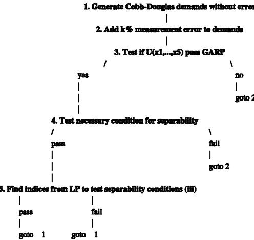
Data generated with measurement error are Žrst tested for consistency with GARP, and thus the existence of a utility function U 4x11 x21 x31 x41 x55 using Varian’s transitive clo-sure test, Equation (3). If the data satisfy GARP, we then test if the Žrst three goods are separable from the remaining goods U 4V 4y51 x41 x55, where yD4x11 x21 x35. This requires two steps. First, the transitive closure test is applied to the subutil-ity functionV 4y5which must also satisfy GARP, the necessary condition for weak separability. Second, given a dataset that satisŽes the necessary condition, we use our LP approach to get estimates for 1=Œi _andVi_{to evaluate Varian’s separability}

condition (iii). Finally, we examine how much adjustment to the superlative index numbersvi _andŒi _{is required for them}

to satisfy the separability conditions. Figure 1 illustrates the Monte Carlo procedure.

5.1 GARP Tests of Utility Maximization

The data are Žrst tested for consistency with GARP using Varian’s (1982) method for calculating the transitive closure,

Figure 1. Steps of the Monte Carlo Experiment.

Table 1. GARP Tests of the Afriat Inequalities

Proportion of data consistent with GARP

Meas. error (K) 1% 5% 10% 20%

Pref._A °

A 0997 0877 0690 0406

°

B 10000 0800 0539 0212

°_C 10000 0941 0570 0151

Pref._B °

A 0997 0830 0611 0414

°

B 0997 0794 0423 0168

°

C 10000 0921 0459 0085

Tests using transitive closure method record a violation whenmt_{i j}D1 andpj_xj_>pj_xi_for

someiandj; see Equation (3).

Preferences:A2 1D0601 ₂D0251 ₃D0101 ₄D0041 ₅D001._B2 ₁D0401 ₂D0301 ₃D 0151 ₄D0101 ₅D005.

Price distributions:°_A¹uniform[98,100],°_B¹uniform[95,100],°_C¹uniform[90,100].

BD21000 Monte Carlo trials were performed.

applying the algorithm of Warshall. This follows steps 11213 from Figure 1, with results displayed in Table 1. These tests are performed using TSP International version 4.5.

The data satisfy GARP over 99% of the time (see Table 1), and are robust to the price distributions and preferences, when the data have 1% measurement error. With 5% measurement error, the data satisfy GARP between 79.4 and 94.0% of the time. As the measurement error increases to 10%, the data now pass GARP between 42.3 and 69.0% of the time. With 20% measurement error, the data pass GARP between 8.4 and 41.4% of the time. Data generated with preferences_A satisfy GARP more often compared to preferences_B, regardless of the amount of measurement error or price distribution.

The distribution of the number of GARP violations is in Appendix B. The tests using the transitive closure method [Equation (3)] record a violation of GARP whenmtijD1 and

pj_xj_{> p}j_xi _{for some i and j. Thus, each dataset can have}

zero or many violations. Data with 1, 5, and 10% measure-ment error have remarkably few violations, regardless of both the preferences and price distributions, that is, fewer than or equal to six violations more than 96.3% of the time. Even with 20% measurement error, there were fewer than or equal to ten violations over 80% of the time. Thus, the transitive closure method of Varian (1982) for testing GARP shows that mea-surement erroris most often likely to result in relatively few

violations of GARP considering that, with 40 observations,

there can be many violations. Note that Bronars (1987) Žnds that the revealed preference tests has much power against the alternative of random behavior.

5.2 Separability Results Using Linear Program Solution

The LP method for testing separability is only applied when the data with error are found to be consistent with GARP, that is, the data pass the necessary condition in step 4 from Figure 1. Applying the LP test requires using a superlative index to estimate the group quantity index. We use a chained Tørnqvist (1936) index, the discrete-time approximation to the Divisia index, because it can be derived from a constrained consumer optimization, and is also a superlative index; see Diewert (1976, 1978), Barnett (1980), and Barnett, Fisher,

and Serletis (1992). The Tørnqvist index should produce very similar results compared to the Fisher ideal index, although Diewert (1992) provides some theoretical grounds for using the Fisher index. The LP routine from Shazam Version 8.0 is used.

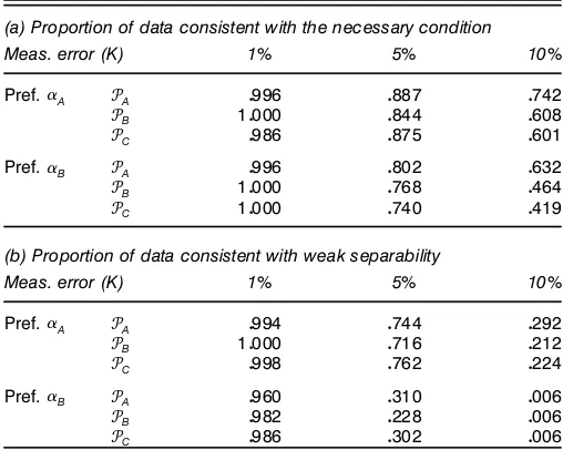
The separability results in Table 2 are in two parts. Since the data often fail to pass GARP with 20% measurement error, tests are performed on data having 1, 5, and 10% measurement error. Table 2(a) examines the proportion of data that satisfy the necessary condition for separability given that the data pass GARP (step 4, Fig. 1). Having passed the necessary condition, Table 2(b) examines the proportion of data that are weakly separable. This is a sufŽcient test, and represents the lower bound of datasets that are consistent with weak separability. Finally, Appendix C gives the cumulative distributions of weak separability.

Table 2(a) shows that the data pass the necessary condi-tion over 98.6% of the time with 1% measurement error, and 74.0–88.7% of the time when there is as much as 5% mea-surement error. With preferences_A(preferences_B) and 10% measurement error, the data satisfy the necessary condition between 60.1 and 74.2% (41.9–63.2%) of the time.

Table 2(b) shows the proportion of data consistent with weak separability. The results are very impressive given that Varian’s NONPAR procedure fails to Žnd separability for Cobb–Douglas demands generated without error; see Barnett and Choi (1989). We also failed to Žnd any datasets weakly separable using NONPAR. With 1% measurement error, the data are consistent with weak separability between 98.2–100% of the time, regardless of the preferences and price distribu-tion. However, with 5% measurement error, weak separability is more likely to be satisŽed with preferences _A (between 71.6 and 76.2%) compared to preferences _B (between 22.8 and 31.0%). Thus, when the data have about 5% measurement error, our LP approach is more likely to Žnd separability when

Table 2. Separability Results

(a) Proportion of data consistent with the necessary condition

Meas. error (K) 1% 5% 10%

Pref._A °

A 0996 0887 0742

°

B 10000 0844 0608

°

C 0986 0875 0601

Pref._B °

A 0996 0802 0632

°

B 10000 0768 0464

°

C 10000 0740 0419

(b) Proportion of data consistent with weak separability

Meas. error (K) 1% 5% 10%

Pref._A °

A 0994 0744 0292

°_B 10000 0716 0212

°

C 0998 0762 0224

Pref.B °A 0960 0310 0006

°

B 0982 0228 0006

°

C 0986 0302 0006

Tests using transitive closure method record a violation whenmtijD1 and pjxj>pjxifor

someiandj.

Preferences:A2 1D060,₂D025,₃D010,₄D004,₅D001._B2 ₁D040,₂D030,

₃D015,₄D010,₅D005.

Price distributions:°_A¹uniform[98,100],°_B¹uniform[95,100],°_C¹uniform[90,100].

BD21000 Monte Carlo trials were performed.

consumers have preferences A, which are often the case in

consumer studies. It is important to note that these results show the minimum proportion of datasets that are consistent with weak separability.

Finally, Appendix C gives the cumulative distributions of the weak separability tests. Once again, there are remarkably few violations with 1% measurement error where over 99% of all the datasets have two or fewer violations, regardless of the preferences or price distribution. With 5% measurement error, over 67.6% of the datasets have eight or fewer viola-tions, again regardless of the preferences or price distribution. The number of violations of weak separability increases when the measurement error is 10%. Given considerable measure-ment error, the number of datasets having ten or fewer viola-tions drops to over 68% for preference A and only 7% for

preference setting_B.

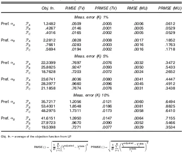
5.3 Superlative Index, Separability, and Measurement Error

When the data are measured with error, a small adjustment to a superlative index may be required to satisfy weak sep-arability. In this study, the superlative index is the Tørnqvist index. Table 3 is used to evaluate how large the adjusted Tørn-qvist with error differs from the TørnTørn-qvist index calculated from the data. Table 3 gives the average of the objective func-tion, the root mean square error (RMSE), and the percentage root mean square error (PRMSE) from the datasets that pass weak separability. Note that the Tørnqvist index calculated from the data was normalized to equal 100 at the Žrst obser-vation. Recall that the objective function minimizes the devi-ations around the group quantity index and the inverse of the group price index. For completeness, the RMSE and PRMSE are reported for both the quantity and price indexes.

The objective function is relatively small, but is larger when the measurement error is 5 or 10%. Nonetheless, the average of the objective function indicates that the Tørnqvist index requires relatively minor adjustments in order to satisfy the Afriat inequalities for the weakly separable subset. This result is also supported by the average RMSE and PRMSE, which are also relatively small for the all of the datasets. Figure 2 plots the Tørnqvist index calculated from the data [QVi _from

Equation (8)] and the adjusted Tørnqvist index for data4QVüi₅

generated with 10% measurement error and preferenceAand

price distribution°_C.

6. TYPE II ERRORS AND THE LP SEPARABILITY TEST

We now turn our attention to the ability of our test to reject weak separability for data generated from a utility function that is not weakly separable. Before doing so, it should be pointed out that any dataset that passes our LP weak separa-bility test also satisŽes Varian’s (1983) separasepara-bility conditions discussed in Section 1. The converse, however, is not nec-essarily true. Note that if the observed quantities and prices satisfy Varian’s (1983) weak separability conditions, then the data can be rationalized by a weakly separable utility function, regardless of how the data were generated.

Table 3. Weak Separability and the Tørnqvist Index: Average Statistics

Obj. fn. RMSE (TV) PRMSE (TV) RMSE (MU) PRMSE (MU)

Meas. error (K) 1%

Pref._A °

A 103482 00509 00005 00006 .0612

°_B 04267 00146 00001 00005 .0529

°

C 04016 00165 00002 00005 .0529

Pref.B °A 202812 00828 00008 00017 .1852

°

B 07661 00283 00003 00016 .1763

°

C 05694 00194 00002 00016 .1718

Meas. error (K) 5%

Pref._A °

A 2203399 07697 00076 00032 .3472

°_B 2508825 09247 00093 00050 .5433

°

C 1807628 07203 00072 00024 .2652

Pref.B °A 2306741 08036 00080 00041 .4447

°

B 2803977 09660 00096 00045 .4912

°

C 2101858 07674 00076 00031 .3438

Meas. error (K) 10%

Pref._A °

A 3507217 102056 00121 00060 .6494

°_B 5304001 108548 00186 00081 .8825

°

C 4802975 107311 00173 00058 .6410

Pref.B °A 4106151 103950 00147 00064 .7155

°

B 2709723 09670 00090 00052 .5466

°

C 1905398 07271 00077 00029 .3534

Obj. fn.Daverage of the objection function from LP.

RMSE(¢)D v u u t 1

B

B

X

iD1 ³

Y_iadjustedƒYdata

i

´2

PRMSE(¢)D v u u t1

B

B

X

iD1 Á

Y_iadjustedƒYdata

i

Ydata

i

!2

TVDTørnqvist index,MUDdeviation from mu,BD2,000 Monte Carlo trials were performed.

To evaluate the probability of a Type II error, we use the utility function of Blackorby, Russell, and Primont (1995) which matches up well with the Monte Carlo experiment in Section 6:

U 4x₁1 x₂1 x₃1 x₄5Dx1=3 1 x

1=3 3 x

1=3 4 Cx

1=2 2 x

1=4 3 x

1=4 4 0

Figure 2. Tørnqvist Index Calculated From the Data and Adjusted Tørnqvist With 5 and 10% Measurement Error.

Their utility function is weakly separable in the goodsx3 and x4 as there exists a subutility functionV 6x31 x47such that

U 4x11 x21 V 6x31 x475Dx 1=3 1 u2Cx

1=2 2 u

3=4 2 1

where

u2DV 6x31 x47Dx 1=3 3 x

1=3 4 0

However, the group of goods x1 andx2 are not weakly

sep-arable from x3 and x4, and thus there is NO subutility

func-tionH 6x11 x27such that their utility function can be written as

U 4x31 x41 H 6x11 x275. The type II error for the Blackorby et al.

utility function is as follows.

Type II Error. Fail to reject the null that the data are sep-arable when the nullH₀2 U 4x₃1 x₄1 H 6x₁1 x₂75is false.

The Monte Carlo experiment is the same as outlined in Figure 1 using the Blackorby et al. (1995) utility function U 4x11 x21 x31 x45. First, we use the transitive closure test of

Varian (1992) to test if data are consistent with GARP. Using the GARP consistent data, the transitive closure test of Varian (1982) is then used to evaluate the necessary conditions for the subutility functionH 6x11 x27. Weak separability for a type

II error is then evaluated using only datasets that pass the necessary condition forH 6x₁1 x₂7.

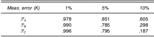
Table 4 shows that the Blackorby et al. (1995) data satisfy GARP forU 4x11 x21 x31 x45over 97.8% of the time, and are

Table 4. Proportion of Data Consistent with GARPU(x1,x2,x3,x4)for

Blackorby et al. (1995)

Meas. error (K) 1% 5% 10%

°_A .978 .851 .605

°_B .990 .785 .298

°_C .996 .795 .187

Price distributions:°_A¹uniform[98,100],°_B¹uniform[95,100].°_C¹uniform[90,100]. BD2,000 Monte Carlo trials were performed.

robust to the price distributions when the data have 1% mea-surement error. With 5% meamea-surement error, the data satisfy GARP between 78.5 and 85.1% of the time. As the measure-ment error increases to 10%, the data pass GARP between 18.7 and 60.5% of the time.

Type II Error Results. Results for the nonseparable utility

functionU 4x31 x41 H 6x11 x275are in Table 5. From Table 5(a),

results show that the probability that the data for the subutil-ity functionH 6x11 x27 are consistent with the necessary

con-dition for weak separability are between (87.7 and 93.8% for 1% measurement error), (44.0 and 67.1% for 5% mea-surement error), and (10.6 and 40.8% for 10% meamea-surement error).

The test results for the nonseparable utility function U 4x31 x41 H 6x11 x275are in Table 5(b), and use only the data

that pass the necessary condition for weak separability for H 6x11 x27. Note that Table 5(b) shows the probability of

reject-ing the false null for the Blackorby et al. (1995) utility function, given that the data pass the necessary condition for H 6x11 x27. For data generated with 5 and 10% error, the false

null is rejected with a probability of 1, regardless of the price distribution. With 1% measurement error, the false null is rejected between 55.0 and 68.3% of the time, regardless of the price distribution.

Finally, any weak separability test should unambiguously reject weak separability for data that fail to pass the

nec-Table 5. GARP Tests of the Afriat Inequalities for the Utility Function of Blackorby et al. (1995)*

(a) GARP necessary condition testsH[x11x2]

Meas. error (K) 1% 5% 10%

°_A 0925 0671 0408

°

B 0877 0440 0181

°

C 0938 0676 0106

(b) Weak separability tests: Probability of rejecting the false null:H02U(x31x41H[x11x2])

Meas. error (K) 1% 5% 10%

°_A 0550 10000 10000

°

B 0617 10000 10000

°

C 0683 10000 10000

ü_H[x

11x2]Dnonseparable data.

Price distributions:°_A¹uniform[98,100],°_B¹uniform[95,100],°_C¹uniform[90,100].

BD2,000 Monte Carlo trials were performed.

Table 6. Separability Results for Monetary Dataa

Sample Violations PRMSE (TV ) PRMSE (MU)

70:1–85:2 2 00868 106177

70:1–79:4 0 00336 04011

75:3–85:2 0 00372 02717

a_{The data are nondurables, services, leisure, currency, demand deposits, other checkable}

deposits, and savings deposits and preferences U2 (ndur, ser, leis, std V(om1, ocd, sd); see Swofford and Whitney (1994, Table 3) for more details.

essary weak separability condition for H 6x11 x27. Using data

that fail to pass the necessary condition, the new LP test cor-rectly rejects the false null of separability with probability 1, regardless of the price distribution. Moreover, we never even Žnd an LP solution, so there was indeed no solution for Theorem 1.

7. APPLICATION USING MONETARY DATA

In testing the necessary and sufŽcient conditions for weak separability, Swofford and Whitney (1994) use quarterly mon-etary data over the period 1970:1 through 1985:2. However, due to computational constraints, they had to use two overlap-ping subsamples. We perform our test over the entire sample and both subsamples. The results appear in Table 6, and are the same as the results from the supercomputer. Swofford and Whitney (1994) were not able to test weak separability over the entire sample, and hence the importance of our PC-based test. However, we fail to Žnd that the data are weakly separa-ble over the entire sample.

8. CONCLUSION

This article derives a new method, which can be used on a PC, for testing for global weak separability. The results show a considerable improvement over existing approaches to empiri-cally evaluate revealed preference separability tests. Moreover, our approach provides a solution that has an economic inter-pretation. The results are based on three different price dis-tributions (relative prices can vary between periods between 4.1% and as much as 23.5%), two sets of preferences typically found in consumer studies, and different amounts of measure-ment error (1, 5, 10, and 20%).

The main results are as follows.

(1) Datasets generated from consumers with preferences most likely to be found in empirical studies pass the neces-sary condition for weak separability over 98 and 84.4% of the time when there is a 1 or 5% measurement error, respectively. (2) Given that a dataset with 1% measurement error satis-Žes the necessary condition, our tests Žnds weak separabil-ity over 96% of the time, regardless of the price distribution or preferences. With 5 and 10% measurement error, data are weakly separable over 71 and 21% of the time, respectively, with preferencesA.

(3) The false null of weak separability, when the generated data are nonseparable, is rejected with a probability of 1 for data simulated with 5 and 10% error. With 1% measurement error, the false null is rejected between 55.0 and 68.3% of the time.

(4) A superlative index number like the Tørnqvist, which is the discrete-time approximation to the Divisia index, when calculated from observed data, needs relatively minor adjust-ments to satisfy Afriat separability inequalities, and hence to provide a ranking of market bundles consistent with the axioms of revealed preference.

(5) GARP is relatively robust to measurement error. For a measurement error of up to 5%, there are often no violations of GARP. When there is a considerable measurement error of 20%, the data often fail to pass GARP, but have relatively few violations.

(6) Measurement error generally produces relatively few violations of GARP and weak separability, and thus, surpris-ingly, measurement error may not be the likely source of the rejection when there are many violations.

(7) Using our procedure that can readily be run on a PC, we conŽrm the separability results obtained by Swofford and Whitney (1994) whose used a CRAY supercomputer.

ACKNOWLEDGMENTS

A. R. Fleissig acknowledges the support of CSFU Untenured Faculty Development Program Grants. The authors thank Jeffery Wooldridge, the associate editor, and two anonymous referees for many helpful suggestions.

APPENDIX A

To convert the nonstandard LP form, substitute Equation (13) into Equations (10) and (16), and rearrange the equations, which gives the LP model instandard form.

Theorem 2. LP Solution for Separability:Standard Form

Minimize ZD

The optimal solution gives nonnegative values for Qi p, Q

n. Note that, if the optimal solution is nonzero, then

at least one4Qi

ate the separability condition (iii).

Example for LP Setup with Three Goods and Three Obser-vations:

APPENDIX B: CUMULATIVE DISTRIBUTION FOR VIOLATIONS OF GARP

1) PreferenceA

Meas. error 1% 5%

°

A °B °C °A °B °C

vD0 099668 1000000 1000000 087742 087995 0094062

vµ2 1000000 098968 099010 0099865

vµ4 099871 1000000 0099865

vµ6 1000000 1000000

Meas. error 10% 20%

°

A °B °C °A °B °C

vD0 068995 053943 057037 040594 021192 015135

vµ2 093612 086745 087986 075248 050047 041014

vµ4 098126 094883 096339 088366 070577 058784

vµ6 099319 098154 099027 097277 084957 072770

vµ8 099830 099413 099828 099010 090634 082635

vµ10 1000000 099832 099943 099505 094891 089662

vµ12 099832 1000000 099752 098202 094459

vµ14 099832 1000000 099432 097027

vµ16 099916 099716 098716

vµ18 1000000 099905 099054

vµ20 1000000 099459

vµ22 099595

vµ24 099662

vµ26 099865

vµ28 099932

vµ30 099932

vµ32 1000000

Tests using transitive closure method record a violation whenmti jD1 andpjxj>pjxifor

someiandj.

vDnumber of GARP violations.

Preferences:A2 1D060,₂D025,₃D010,₄D004,₅D001._B2 ₁D040,₂D030,

3D015,₄D010,₅D005.

Price distributions:°_A¹uniform[98,100],°_B¹uniform[95,100],°_C¹uniform[90,100].

2) Preference_B

Meas. error 1% 5%

°_A °_B °_C °_A °_B °_C

vD0 099668 099668 1000000 082960 079351 092132

vµ2 1000000 1000000 098206 097738 099365

vµ4 099776 099508 099873

vµ6 1000000 099902 1000000

vµ8 1000000

Meas. error 10% 20%

°

A °B °C °A °B °C

vµ0 061100 042314 045868 041438 016838 008522

vµ2 090007 077478 078067 076541 043190 024973

vµ4 096512 090984 090909 091781 066119 042233

vµ6 098860 096857 096281 096918 079124 057389

vµ8 099531 098791 098347 099315 088843 069471

vµ10 099665 099482 099237 099829 093840 080288

vµ12 099866 099793 099746 1000000 097194 085922

vµ14 099933 099931 099968 098563 091100

vµ16 1000000 099965 1000000 099247 094391

vµ18 1000000 099726 096548

vµ20 099863 097465

vµ22 099932 098382

vµ24 1000000 099029

vµ26 099245

vµ28 099299

vµ30 099461

vµ32 099784

vµ34 099838

vµ36 099838

vµ38 099892

vµ40 099946

vµ42 099946

vµ44 099946

vµ46 099946

vµ48 1000000

Tests using transitive closure method record a violation whenmt_{i j}D1 andpj_xj_>pj_xi_for

someiandj.

vDnumber of GARP violations.

Preferences:_A2 1D060,₂D025,₃D010,₄D004,₅D001.

B2 1D040,₂D030,

3D015,₄D010,₅D005.

Price distributions:°_A¹uniform[98,100],°_B¹uniform[95,100],°

C¹uniform[90,100].

APPENDIX C: CUMULATIVE DISTRIBUTION FOR VIOLATIONS OF WEAK SEPARABILITY

1) PreferenceA

Meas. error 1%

°

A °B °C

vD0 099400 100000 099800

vµ2 099800 1000000

vµ4 099800

vµ6 1000000

Meas. error 5% 10%

°

A °B °C °A °B °C

vD0 074400 071600 076200 029200 021200 022400

vµ2 092400 088800 090400 055200 042400 040600

vµ4 095600 092000 092600 064800 051600 048800

vµ6 097800 094200 094200 071600 058400 057600

vµ8 098600 095800 095600 077000 064000 062000

vµ10 099600 096800 095800 080000 068000 068200

vµ12 099600 097400 096200 082400 072200 072000

vµ14 099800 097800 096800 085600 075000 075800

vµ16 099800 098200 097600 087800 076800 078800

vµ18 1000000 098200 097800 088800 079000 080600

vµ20 098200 097800 089400 080400 082000

vµ22 098400 098200 090000 082400 082400

vµ24 098600 098200 090800 083600 082600

vµ26 098800 098200 091000 085600 082600

vµ28 099000 098400 092000 086600 084600

vµ30 099000 098600 092600 086800 085000

vµ32 099200 098800 092800 087600 085400

vµ34 099400 098800 093200 088000 086000

vµ36 099600 098800 093200 088400 086600

vµ38 099600 099000 093400 088600 087200

vµ40 099800 099000 093400 088600 087800

vµ42 1000000 099200 093800 088800 088200

vµ44 099200 094000 089400 088400

vµ46 099200 094200 089600 088600

vµ48 099400 094400 089800 088800

vµ50 099400 094600 090400 089400

Tests using transitive closure method record a violation whenmti jD1 andpjxj>pjxifor

someiandj.

vDnumber of GARP violations.

Preferences:_A2 ₁D0601 ₂D0251 ₃D0101 ₄D0041 ₅D001._B2 ₁D0401 ₂D0301 ₃D 0151 4D0101 5D005.

Price distributions:°_A¹uniform[98,100],°_B¹uniform[95,100],°_C¹uniform[90,100].

2) Preference_B

Meas. error 1%

°_A °_B °_C

vD0 096000 098200 098600

vµ2 099800 099600 099600

vµ4 099800 1000000 099800

vµ6 1000000 1000000

Meas. error 5% 10%

°

A °B °C °A °B °C

vD0 031000 022800 030200 000600 000600 000600

vµ2 052600 043000 051800 003800 001000 001800

vµ4 062200 054200 060200 007200 001800 002800

vµ6 071200 062200 065800 010600 003600 003800

vµ8 078800 067600 070400 014400 006000 006000

vµ10 083000 072600 075200 019400 008000 007000

vµ12 085600 076400 079000 024600 011200 008400

vµ14 088800 080000 082200 030000 013200 009800

vµ16 090200 082800 083800 033800 016200 011200

vµ18 091400 083800 085400 037200 018400 013000

vµ20 092800 085600 086000 040400 020200 014600

vµ22 094000 086600 087400 043000 022600 016200

vµ24 094800 087600 088800 045000 024200 018200

vµ26 095200 088800 089400 047600 026000 020600

vµ28 095600 089800 089800 049000 028000 022600

vµ30 095800 090600 090000 052000 029200 023800

vµ32 096400 091200 090400 053800 030400 024400

vµ34 096400 091200 090800 055600 032200 026000

vµ36 096800 091600 091600 058200 033600 027600

vµ38 096800 092200 091800 059200 035000 028600

vµ40 096800 092400 092800 061000 036400 029800

vµ42 097400 093400 093200 062600 037800 030800

vµ44 097800 094000 093600 064200 039400 031800

vµ46 098000 094000 093800 065200 040400 032800

vµ48 098000 094200 094000 066600 041800 034000

vµ50 098000 094400 094400 067000 043000 035400

vµ52 098000 094400 094600 068600 044600 036000

vµ54 098400 094800 095000 070000 046200 037600

vµ56 098400 094800 095000 070600 047000 038400

vµ58 098400 095200 095200 072200 048000 038600

vµ60 098400 095600 095400 073600 048200 039000

vµ62 098400 095600 095600 074200 048400 039200

vµ64 098600 095800 095600 074400 049400 040400

vµ66 098800 096400 095800 074800 050200 041200

vµ68 098800 096400 095800 074800 051000 042400

vµ70 098800 096400 096000 075600 051800 043400

vµ82 098800 096400 096200 076000 053000 044400

vµ84 099000 096400 096600 077000 054400 044600

vµ86 099000 096600 096800 077600 054400 045200

vµ88 099000 096800 097000 078000 054600 045400

vµ90 099000 097200 097000 079000 054800 046400

vµ92 099000 097600 097000 079400 055400 046600

vµ94 099200 097800 097000 080200 056400 047000

vµ96 099400 097800 097000 081000 058400 048000

vµ98 099400 098000 097000 081200 060400 048400

vµ100 099400 098000 097000 081200 060800 049600

Tests using transitive closure method record a violation whenmti jD1 and pjxj>pjxi, for

someiandj.

vDnumber of GARP violations.

Preferences:A2 1D0601 2D0251 3D0101 4D0041 5D001._B2 1D0401 2D0301 3D 0151 ₄D0101 ₅D005.

Price distributions:°_A¹uniform[98,100],°_B¹uniform[95,100],°_C¹uniform[90,100].

[Received April 2000. Revised March 2001.]

REFERENCES

Afriat, S. (1967), “The Construction of a Utility Function From Expenditure Data,”International Economic Review, 8, 67–77.

Barnett, W. A., and Choi, S. (1989), “A Monte Carlo Study of Tests of Block-wise Weak Separability,”Journal of Business and Economics Statistics, 7, 363–377.

Barnett, W. A. (1980), “Economic Monetary Aggregates: An Application of Index Number Theory and Aggregation Theory,”Journal of Econometrics, 14, 11–48.

Barnett, W. A., Fisher, D., and Serletis, A. (1992), “Consumer Theory and the Demand for Money,”Journal of Economic Literature, 4, 2086–2119. Bronars, S. G. (1987), “The Power of Nonparametric Tests of Preference

Maximization,”Econometrica, 55, 693–698.

Brown, B. W., and Walker, M. B. (1989), “The Random Utility Hypothesis and Inference in Demand Systems,”Econometrica, 57, 815–829. Chalfant, J. A., and Alston, J. M. (1988), “Accounting for Changes in Tastes,”

Journal of Political Economy, 96, 391–410.

Diewert, W. E. (1973), “Afriat and Revealed Preference Theory,”The Review of Economic Studies, 40, 419–426.

(1976), “Exact and Superlative Index Numbers,”Journal of Econo-metrics, 4, 115–145.

(1978), “Superlative Index Numbers and Consistency in Aggregation,”

Econometrica, 46, 883–900.

(1992), “Fisher Ideal Output, Input and Productivity Indexes Revis-ited,”Journal of Productivity Analysis, 3, 211–248.

Diewert, W. E., and Wales T. J. (1995), “Flexible Functional Forms and Tests of Homogeneous Separability,”Journal of Econometrics, 67, 259–302. Epstein, L. G., and Yatchew, A. J. (1985), “Non-Parametric Hypothesis

Test-ing Procedures and Applications to Demand Analysis,”Journal of Econo-metrics, 30, 149–169.

Fleissig, A. R., Hall, A., and Seater, J. J. (2000), “GARP, Separability and the Representative Agent,”Macroeconomic Dynamics, 4, 324–342. Fleissig, A. R., and Swofford, J. (1996), “A Dynamic Asymptotically Ideal

Model of Money Demand,”Journal of Monetary Economics, 37, 371–380. Gross, J. (1991), “On Expenditure Indices in Revealed Preference Tests,”

Journal of Political Economy, 99, 416–419.

(1995), “Testing Data for Consistency With Revealed Preference,”

The Review of Economics and Statistics, 77, 701.

Gross J., and Kaiser D. (1996), “Two Simple Algorithms for Generating a Subset of Data Consistent With WARP and Other Binary Relations,” Jour-nal of Business and Economics Statistics, 14, 251–255.

Houthakker, H. (1950), “Revealed Preference and the Utility Function,” Eco-nomica, 17, 159–174.

Manser, M. E., and McDonald, R. J. (1988), “An Analysis of Substitution Bias in Measuring Ination, 1959–85,”Econometrica, 56, 909–930. Richter, M. (1966), “Revealed Preference Theory,”Econometrica, 34, 635–645. Samuelson, P. A. (1948), “Consumption Theory in Terms of Revealed

Pref-erence,”Economica, 15, 243–253.

Swofford, J. L., and Whitney, G. A. (1987), “Non-Parametric Tests of Util-ity Maximization and Weak SeparabilUtil-ity for Consumption, Leisure and Money,”Review of Economics and Statistics, 69, 458–464.

(1988), “A Comparison of Non-Parametric Tests of Weak Separability for Annual and Quarterly Data on Consumption, Leisure, and Money,”

Journal of Business and Economics Statistics, 6, 241–246.

(1994), “A Revealed Preference Test for Weakly Separable Utility Maximization With Incomplete Adjustment,”Journal of Econometrics, 60, 235–249.

Tørnqvist, L. (1936), “The Bank of Finland’s Consumption Price Index,”Bank of Finland Monthly Bulletin, 10, 1–8.

Varian, H. (1982), “The Nonparametric Approach to Demand Analysis,”

Econometrica, 50, 945–973.

(1983), “Nonparametric Tests of Consumer Behavior,”Review of Eco-nomic Studies, 50, 99–110.

(1985), “Non-Parametric Analysis of Optimizing Behavior With Mea-surement Error,”Journal of Econometrics, 30, 445–458.