CAMBRIDGE MONOGRAPHS ON
APPLIED AND COMPUTATIONAL
MATHEMATICS
Series Editors
P. G. CIARLET, A. ISERLES, R. V. KOHN, M. H. WRIGHT
crucial role of mathematical and computational techniques in contemporary science. The series publishes expositions on all aspects of applicable and numerical mathematics, with an emphasis on new developments in this fast-moving area of research.
State-of-the-art methods and algorithms as well as modern mathematical descriptions of physical and mechanical ideas are presented in a manner suited to graduate research students and professionals alike. Sound pedagogical presentation is a prerequisite. It is intended that books in the series will serve to inform a new generation of researchers.
Also in this series:
1. A Practical Guide to Pseudospectral Methods,Bengt Fornberg
2. Dynamical Systems and Numerical Analysis,A. M. Stuart and A. R. Humphries
3. Level Set Methods and Fast Marching Methods,J. A. Sethian
4. The Numerical Solution of Integral Equations of the Second Kind,Kendall E. Atkinson
5. Orthogonal Rational Functions,Adhemar Bultheel, Pablo Gonz´alez-Vera, Erik Hendiksen, and Olav Nj˚astad
6. The Theory of Composites,Graeme W. Milton
7. Geometry and Topology for Mesh Generation,Herbert Edelsbrunner
8. Schwarz–Christoffel Mapping,Tofin A. Driscoll and Lloyd N. Trefethen
9. High-Order Methods for Incompressible Fluid Flow,M. O. Deville, P. F. Fischer, and E. H. Mund
10. Practical Extrapolation Methods,Avram Sidi
11. Generalized Riemann Problems in Computational Fluid Dynamics,Matania Ben-Artzi and Joseph Falcovitz
12. Radial Basis Functions: Theory and Implementations,Martin D. Buhmann
13. Iterative Krylov Methods for Large Linear Systems,Henk A. van der Vorst
14. Simulating Hamiltonian Dynamics,Ben Leimkuhler and Sebastian Reich
15. Collocation Methods for Volterra Integral and Related Functional Equations,
Topology for Computing
AFRA J. ZOMORODIAN
Cambridge, New York, Melbourne, Madrid, Cape Town, Singapore, São Paulo
Cambridge University Press
The Edinburgh Building, Cambridge , UK
First published in print format
- ---- - ---- © Afra J. Zomorodian 2005
Information on this title: www.cambridge.org/9780521836661
This book is in copyright. Subject to statutory exception and to the provision of relevant collective licensing agreements, no reproduction of any part may take place without the written permission of Cambridge University Press.
- ---
- ---
Cambridge University Press has no responsibility for the persistence or accuracy of s for external or third-party internet websites referred to in this book, and does not guarantee that any content on such websites is, or will remain, accurate or appropriate. Published in the United States of America by Cambridge University Press, New York www.cambridge.org
hardback
eBook (NetLibrary) eBook (NetLibrary)
—Persistence of Homology—Afra Zomorodian (After Salvador Dali)
To my parents
Contents
Preface pagexi
Acknowledgments xiii
1 Introduction 1
1.1 Spaces 1
1.2 Shapes of Spaces 3
1.3 New Results 8
1.4 Organization 10
Part One: Mathematics
2 Spaces and Filtrations 13
2.1 Topological Spaces 14
2.2 Manifolds 19
2.3 Simplicial Complexes 23
2.4 Alpha Shapes 32
2.5 Manifold Sweeps 37
3 Group Theory 41
3.1 Introduction to Groups 41
3.2 Characterizing Groups 47
3.3 Advanced Structures 53
4 Homology 60
4.1 Justification 60
4.2 Homology Groups 70
4.3 Arbitrary Coefficients 79
5 Morse Theory 83
5.1 Tangent Spaces 84
5.2 Derivatives and Morse Functions 85
5.3 Critical Points 86
5.4 Stable and Unstable Manifolds 88
5.5 Morse-Smale Complex 90
viii
6 New Results 94
6.1 Persistence 95
6.2 Hierarchical Morse-Smale Complexes 105
6.3 Linking Number 116
Part Two: Algorithms
7 The Persistence Algorithms 125
7.1 Marking Algorithm 125
7.2 Algorithm forZ2 128
7.3 Algorithm for Fields 136
7.4 Algorithm for PIDs 146
8 Topological Simplification 148
8.1 Motivation 148
8.2 Reordering Algorithms 150
8.3 Conflicts 153
8.4 Topology Maps 157
9 The Morse-Smale Complex Algorithm 161
9.1 Motivation 162
9.2 The Quasi Morse-Smale Complex Algorithm 162
9.3 Local Transformations 166
9.4 Algorithm 169
10 The Linking Number Algorithm 171
10.1 Motivation 171
10.2 Algorithm 172
Part Three: Applications
11 Software 183
11.1 Methodology 183
11.2 Organization 184
11.3 Development 186
11.4 Data Structures 190
11.5 CView 193
12 Experiments 198
12.1 Three-Dimensional Data 198
12.2 Algorithm forZ2 204
12.3 Algorithm for Fields 208
12.4 Topological Simplification 215 12.5 The Morse-Smale Complex Algorithm 217 12.6 The Linking Number Algorithm 220
13 Applications 223
Contents
ix
13.3 Denoising Density Functions 229
13.4 Surface Reconstruction 231
13.5 Shape Description 232
13.6 I/O Efficient Algorithms 233
Bibliography 235
Index 240
Preface
My goal in this book is to enable a non-specialist to grasp and participate in current research in computational topology. Therefore, this book is not a compilation of recent advances in the area. Rather, the book presents basic mathematical concepts from a computer scientist’s point of view, focusing on computational challenges and introducing algorithms and data structures when appropriate. The book also incorporates several recent results from my doc-toral dissertation and subsequent related results in computational topology.
The primary motivation for this book is the significance and utility of topo-logical concepts in solving problems in computer science. These problems arise naturally in computational geometry, graphics, robotics, structural biol-ogy, and chemistry. Often, the questions themselves have been known and considered by topologists. Unfortunately, there are many barriers to interac-tion:
• Computer scientists do not know the language of topologists. Topology,
unlike geometry, is not a required subject in high school mathematics and is almost never dealt with in undergraduate computer science. The axiomatic nature of topology further compounds the problem as it generates cryptic and esoteric terminology that makes the field unintelligible and inaccessible to non-topologists.
• Topology can be very unintuitive and enigmatic and therefore can appear
very complicated and mystifying, often frightening away interested com-puter scientists.
• Topology is a large field with many branches. Computer scientists often
re-quire only simple concepts from each branch. While there are certainly a number of offerings in topology by mathematics departments, the focus of these courses is often theoretical, concerned with deep questions and exis-tential results.
Because of the relative dearth of interaction between topologists and computer scientists, there are many opportunities for research. Many topological ques-tions have large complexity: the best known bound, if any, may be exponential. For example, I once attended a talk on an algorithm that ran in quadruply ex-ponential time! Let me make this clear. It was
O
2222
n
.
And one may overhear topologists boasting that their software can now han-dle 14 tetrahedra, not just 13. But better bounds may exist for specialized questions, such as problems in low dimensions, where our interests chiefly lie. We need better algorithms, parallel algorithms, approximation schemes, data structures, and software to solve these problems within our lifetime (or the lifetime of the universe.)
This book is based primarily on my dissertation, completed under the super-vision of Herbert Edelsbrunner in 2001. Consequently, some chapters, such as those in Part Three, have a thesis feel to them. I have also incorporated notes
from several graduate-level courses I have organized in the area:Introduction
to Computational Topologyat Stanford University, California, during Fall 2002
and Winter 2004; andTopology for Computingat the Max-Planck-Institut für
Informatik, Saarbrücken, Germany, during Fall 2003.
The goal of this book is to make algorithmically minded individuals fluent in the language of topology. Currently, most researchers in computational topol-ogy have a mathematics background. My hope is to recruit more computer scientists into this emerging field.
Stanford, California A. J. Z.
Acknowledgments
I am indebted to Persi Diaconis for the genesis of this book. He attended my very first talk in the Stanford Mathematics Department, asked for a copy of my thesis, and recommended it for publication. To have my work be recognized by such a brilliant and extraordinary figure is an enormous honor for me. I would like to thank Lauren Cowles for undertaking this project and coaching me throughout the editing process and Elise Oranges for copyediting the text.
During my time at Stanford, I have collaborated primarily with Leonidas Guibas and Gunnar Carlsson. Leo has been more than just a post-doctoral supervisor, but a colleague, a mentor, and a friend. He is a successful aca-demic who balances research, teaching, and the mentoring of students. He guides a large animated research group that works on a manifold of significant problems. And his impressive academic progeny testify to his care for their success.
Eleven years after being a freshman in his “honors calculus,” I am fortu-nate to have Gunnar as a colleague. Gunnar astounds me consistently with his knowledge, humility, generosity, and kindness. I continue to rely on his estimation, advice, and support.
I would also like to thank the members of Leo and Gunnar’s research groups as well as the Stanford Graphics Laboratory, for inspired talks and invigorating discussions. This book was partially written during a four-month stay at the Max-Planck-Institut. I would like to thank Lutz Kettner and Kurt Mehlhorn for their sponsorship, as well as for coaxing me into teaching a mini-course.
Finally, I would like to thank my research collaborators, whose work ap-pears in this book: Gunnar Carlsson, Anne Collins, Herbert Edelsbrunner, Leonidas Guibas, John Harer, and David Letscher. My research was sup-ported, in part, by ARO under grant DAAG55-98-1-0177, by NSF under grants CCR-00-86013 and DMS-0138456, and by NSF/DARPA under grant CARGO 0138456.
1
Introduction
The focus of this book is capturing and understanding the topological prop-erties of spaces. To do so, we use methods derived from exploring the re-lationship between geometry and topology. In this chapter, I will motivate this approach by explaining what spaces are, how they arise in many fields of inquiry, and why we are interested in their properties. I will then introduce new theoretical methods for rigorously analyzing topologies of spaces. These methods are grounded in homology and Morse theory, and generalize to high-dimensional spaces. In addition, the methods are robust and fast, and therefore practical from a computational point of view. Having introduced the methods, I end this chapter by discussing the organization of the rest of the book.
1.1 Spaces
Let us begin with a discussion of spaces. Aspaceis a set of points as shown in
Figure 1.1(a). We cannot define what asetis, other than accepting it as a
prim-itive notion. Intuprim-itively, we think of a set as a collection or conglomeration of
objects. In the case of a space, these objects arepoints, yet another primitive
notion in mathematics. The concept of a space is too weak to be interesting, as it lacks structure. We make this notion slightly richer with the addition of atopology. We shall see in Chapter 2 what a topology formally means. Here, we think of a topology as the knowledge of the connectivity of a space: Each
point in the space knows which points are near it, that is, in itsneighborhood.
In other words, we know how the space is connected. For example, in Fig-ure 1.1(b), neighbor points are connected graphically by a path in the graph.
We call such a space atopological space. At first blush, the concept of a
topo-logical space may seem contrived, as we are very comfortable with the richer
metric spaces, as in Figure 1.1(c). We are introduced to the prototypical metric
space, theEuclidean spaceRd, in secondary school, and we often envision our
(a) A space (b) A topological space
0 5 10
5 10
(c) A metric space
Fig. 1.1. Spaces.
world asR3. A metric space has an associatedmetric, which enables us to
measure distances between points in that space and, in turn, implicitly define their neighborhoods. Consequently, a metric provides a space with a topol-ogy, and a metric space is a topological one. Topological spaces feel alien to us because we are accustomed to having a metric. The spaces arise naturally, however, in many fields.
Example 1.1 (graphics) We often model a real-world object as a set of ele-ments, where the elements are triangles, arbitrary polygons, or B-splines.
Example 1.2 (geography) Planetary landscapes are modeled as elevations over
grids, or triangulations, ingeographic information systems.
Example 1.3 (robotics) A robot must often plan a path in its world that con-tains many obstacles. We are interested in efficiently capturing and
represent-ing theconfiguration spacein which a robot may travel.
Example 1.4 (biology) A protein is a single chain of amino acids, which folds
into a globular structure. TheThermodynamics Hypothesisstates that a protein
always folds into a state of minimum energy. To predict protein structure, we would like to model the folding of a protein computationally. As such, the
protein foldingproblem becomes an optimization problem: We are looking for a path to the global minimum in a very high-dimensional energy landscape.
1.2 Shapes of Spaces 3
by focusing on the topology of the space, and not its geometry. I will refer to topological spaces simply as spaces from this point onward.
1.2 Shapes of Spaces
We have seen that spaces arise in the process of solving many problems.
Con-sequently, we are interested in capturing and understanding the shapes of
spaces. This understanding is really in the form of classifications: We would like to know how spaces agree and differ in shape in order to categorize them. To do so, we need to identify intrinsic properties of spaces. We can try trans-forming a space in some fixed way and observe the properties that do not
change. We call these properties the invariants of the space. Felix Klein
gave this famous definition for geometry in hisErlanger Programmaddress
in 1872. For example, Euclidean geometryrefers to the study of invariants
under rigid motion inRd, e.g., moving a cube in space does not change its
geometry. Topology, on the other hand, studies invariants under continuous, and continuously invertible, transformations. For example, we can mold and stretch a play-doh ball into a filled cube by such transformations, but not into a donut shape. Generally, we view and study geometric and topological prop-erties separately.
1.2.1 Geometry
There are a variety of issues we may be concerned with regarding the geometry of a space. We usually have a finite representation of a space for computation. We could be interested in measuring the quality of our representation, trying to improve the representation via modifications, and analyzing the effect of our changes. Alternatively, we could attempt to reduce the size of the representa-tion in order to make computarepresenta-tions viable, without sacrificing the geometric accuracy of the space.
Example 1.5 (decimation) The Stanford Dragon in Figure 1.2(a) consists of 871,414 triangles. Large meshes may not be appropriate for many
applica-tions involving real-time rendering. Havingdecimatedthe surface to 5% of its
(a) Stanford Dragon, rep-resented by a triangulated surface
(b) Decimated to 5% of the number of triangles
(c) Normalized distance to original surface, in in-creasing intensity
Fig. 1.2. Geometric simplification.
Fig. 1.3. The string on the left is cut into two pieces. The loop string on the right is cut but still is in one piece.
1.2.2 Topology
While Klein’s unifying definition makes topology a form of geometry, we of-ten differentiate between the two concepts. Recall that when we talk about topology, we are interested in how spaces are connected. Topology concerns itself with how things are connected, not how they look. Let’s start with a few examples.
Example 1.6 (loops of string) Imagine we are given two pieces of strings. We tie the ends of one of them, so it forms a loop. Are they connected the same way, or differently? One way to find out is to cut both, as shown in Fig-ure 1.3. When we cut each string, we are obviously changing its connectivity. Since the result is different, they must have been connected differently to begin with.
1.2 Shapes of Spaces 5
(a) No matter where we cut the sphere, we get two pieces
(b) If we’re careful, we can cut the torus and still leave it in one piece.
Fig. 1.4. Two pieces or one piece?
piece. Somehow, the torus is acting like our string loop and the sphere like the untied string.
Example 1.8 (holding hands) Imagine you’re walking down a crowded street, holding somebody’s hand. When you reach a telephone pole and have to walk on opposite sides of the pole, you let go of the other person’s hand. Why?
Let’s look back to the first example. Before we cut the string, the two points
near the cut are near each other. We say that they areneighborsor in each
other’sneighborhoods. After the cut, the two points are no longer neighbors,
and their neighborhood has changed. This is the critical difference between the untied string and the loop: The former has two ends. All the points in the loop have two neighbors, one to their left and one to their right. But the untied string has two points, each of whom has a single neighbor. This is why the two strings have different connectivity. Note that this connectivity does not change if we deform or stretch the strings (as if they are made of rubber.) As long as we don’t cut them, the connectivity remains the same. Topology studies this
connectivity, a property that isintrinsicto the space itself.
In addition to studying theintrinsicproperties of a space, topology is
con-cerned not only with how an object is connected (intrinsic topology), but how
it isplacedwithin another space (extrinsic topology.) For example, suppose
we put a knot on a string and then tie its ends together. Clearly, the string has the same connectivity as the loop we saw in Example 1.6. But no matter how we move the string around, we cannot get rid of the knot (in topology terms,
we cannot unknot the knot into theunknot.) Or can we? Can we prove that we
cannot?
Topo-(a) Gramicidin A, a pro-tein, with a tunnel
(b) A knotted DNA (c) Five pairwise-linked tetrahedral skeletons
Fig. 1.5. Topological properties. (b) Reprinted with permission from S Wasserman et al., SCIENCE, 229:171–174 (1985). © 1985 AAAS.
(a) Sampled point set from a surface
(b) Recovered topology (c) Piece-wise linear sur-face approximation
Fig. 1.6. Surface reconstruction.
logical questions arise frequently in many areas of computation. Tools de-veloped in topology, however, have not been used to address these problems traditionally.
Example 1.9 (surface reconstruction) Usually, a computer model is created by sampling the surface of an object and creating a point set, as in Figure 1.6(a).
1.2 Shapes of Spaces 7
Fig. 1.7. Topological simplification.
As for geometry, we would also like to be able to simplify a space topolog-ically, as in Figure 1.7. I have intentionally made the figures primitive com-pared to the previous geometric figures to reflect the essential structure that topology captures. To simplify topology, we need a measure of the importance of topological attributes. I provide one such measure in this book.
1.2.3 Relationship
The geometry and topology of a space are fundamentally related, as they are both properties of the same space. Geometric modifications, such as decima-tion in Example 1.5, could alter the topology. Is the simplified dragon in Fig-ure 1.2(c) connected the same way as the original? In this case, the answer is yes, because the decimation algorithm excludes geometric modifications that have topological impact. We have changed the geometry of the surface without changing its topology.
When creating photo-realistic images, however, appearance is the dominant issue, and changes in topology may not matter. We could, therefore, allow for topological changes when simplifying the geometry. In other words, geometric modifications are possible with, and without, induced changes in topology. The reverse, however, is not true. We cannot eliminate the “hole” in the surface of the donut (torus) to get a sphere in Figure 1.7 without changing the geometry of the surface. We further examine the relationship between topology and geometry by looking at contours of terrains.
Example 1.10 (contours) In Figure 1.8, I show a flooded terrain with the
wa-ter receding. The boundaries of the components that appear are theiso-linesor
Fig. 1.8. Noah’s flood receding.
We may view the spaces shown in Figure 1.8 as a single growing space under-going topological and geometric changes. The history of such a space, called afiltration, is the primary object for this book. Note that the topology of the iso-lines within this history is determined by the geometry of the terrain.
Gen-eralizing to a(d+1)-dimensional surface, we see that there is a relationship
between the topology ofd-dimensionallevel setsof a space and its geometry,
one dimension higher. This relationship is the subject ofMorse theory, which
we will encounter in this book.
1.3 New Results
We will also examine some new results in the area of computational topol-ogy. There are three main groups of theoretical results: persistence, Morse complexes, and the linking number.
1.3 New Results 9
Fig. 1.9. A Morse complex over a terrain.
• Persistence: efficient algorithms for computing persistence over arbitrary coefficients.
• Topological Simplification:algorithms for simplifying topology, based on persistence. The algorithms remove attributes in the order of increasing per-sistence. At any moment, we call the removed attributes topological noise, and the remaining ones topological features.
• Cycles and Manifolds:algorithms for computing representations. The per-sistence algorithm tracks the subspaces that express nontrivial topological attributes, in order to compute persistence. We show how to modify this algorithm to identify these subspaces (cycles), as well as the subspaces that eliminate them (manifolds.)
Morse complexes. A Morse complex gives a full analysis of the behavior of flow over a space by partitioning the space into cells of uniform flow. In the case of a two-dimensional surface, such as the terrain in Figure 1.8, the Morse complex connects maxima (peaks) to minima (pits) through saddle points (passes) via edges, partitioning the terrain into quadrangles, as shown in Figure 1.9. Morse complexes are defined, however, only for smooth spaces. In this book, we will see how to extend this definition to piece-wise linear sur-faces, which are frequently used for computation. In addition, we will learn how to construct hierarchies of Morse complexes.
• Morse complex: We give an algorithm for computing the Morse complex by first constructing a complex whose combinatorial form matches that of the Morse complex and then deriving the Morse complex via local
trans-formations. This construction reflects a paradigm we call theSimulation of
Differentiability.
modifying the geometry of the space in order to eliminate noise and simplify the topology of the contours of the surface.
Linking number. Thelinking numberis an integer invariant that measures the separability of a pair of knots. We extend the definition of the linking number to simplicial complexes. We then develop data structures and algorithms for computing the linking numbers of the complexes in a filtration.
1.4 Organization
The rest of this book is divided into three parts: mathematics, algorithms, and
applications. Part One,Mathematics, contains background on algebra,
geom-etry, and topology, as well as the new theoretical contributions. In Chapter 2, we describe the spaces we are interested in exploring, and how we examine them by encoding their geometries in filtrations of complexes. Chapter 3 pro-vides enough group theory background for the definition of homology groups in Chapter 4. We also discuss other measures of topology and justify our choice of homology. Switching to smooth manifolds, we review concepts from Morse Theory in Chapter 5. In Chapter 6, we give the mathematics behind the new results in this book.
Part Two,Algorithms, contains data structures and algorithms for the
mathe-matics presented in Part I. In each chapter, we motivate and present algorithms and prove they are correct. In Chapter 7, we introduce algorithms for
comput-ing persistence: overZ2coefficients, arbitrary fields, and arbitrary principal
ideal domains. We then address topological simplification using persistence in Chapter 8. In Chapter 9, we describe an algorithm for computing two-dimensional Morse complexes. We end this part by showing how one may compute linking numbers in Chapter 10.
Part Three,Applications, contains issues relating to the application of the
Part One
2
Spaces and Filtrations
In this chapter, we describe the input to all of the algorithms described in this book, and the process by which such input is generated. We begin by formaliz-ing the kind of spaces that we are interested in explorformaliz-ing. Then, we introduce the primary approach used for computing topology: growing a space incre-mentally and analyzing the history of its growth. Naturally, the knowledge we derive from this approach is only as meaningful as the growth process. So, we let the geometry of our space dictate the growth model. In this fashion, we encode geometry into an otherwise topological history. The geometry of our space controls the placement of topological events within this history and, consequently, the life-span of topological attributes. The main assumption of this method is that longevity is equivalent to significance. This approach of exploring the relationship between geometry and topology is not new. It is the
hallmark ofMorse theory(Milnor, 1963), which we will study in more detail
in Chapter 5.
The rest of the chapter describes the process outlined in Figure 2.1. We begin with a formal description of topological spaces. We then describe two types of such spaces, manifolds and simplicial complexes, in the next two sections.
Weighted Point Sets (2.4)
Alpha Shapes (2.4)
Sweep (2.5)
Algorithms
Topological Spaces (2.1)
Filtrations (2.3)
Manifolds (2.2)
Fig. 2.1. Geometrically ordered filtrations: Topics are labeled with their sections.
These spaces constitute our realm of interest. The latter is more general than the former, and we represent the former with it. We also formalize the notion of a growth history (filtration) within Section 2.3. Finally, we describe two growth processes, alpha shapes and manifold sweeps, which are utilized to
spawn filtrations. Thesegeometrically ordered filtrationsprovide the input to
the algorithms.
Topology and algebra are both axiomatic studies, necessitating a large num-ber of definitions. My approach will be to start from the very primitive no-tions, in order to refresh the reader’s memory. The titled definino-tions, however, allow for quick skimming for the knowledgeable reader. My treatment follows Bishop and Goldberg (1980) for point-set topology and Munkres (1984) for algebraic topology. I also used Henle (1997) and McCarthy (1988) for refer-ence and inspiration. I recommend de Berg et al. (1997) for background on computational geometry. I will cite some seminal papers in defining concepts.
2.1 Topological Spaces
A topological space is a set of points who know who their neighbors are. Let’s begin with the primitive notion of a set.
2.1.1 Sets and Functions
We cannot define a set formally, other than stating that asetis a well-defined
collection of objects. We also assume the following:
(i) SetSis made up ofelements a∈S.
(ii) There is only one empty set∅.
(iii) We may describe a set by characterizing it ({x|P(x)}) or by
enumerat-ing elements ({1,2,3}). Here P is a predicate.
(iv) A setSiswell definedif, for each objecta, eithera∈Sora∈S.
Note that “well defined” really refers to the definition of a set, rather than to
the set itself.|S|or cardSis the size of the set. We may multiply sets in order
to get larger sets.
Definition 2.1 (Cartesian) TheCartesian product of sets S1,S2, . . . ,Snis the
set of all orderedn-tuples(a1,a2, . . . ,an), whereai∈Si. The Cartesian
prod-uct is denoted by eitherS1×S2×. . .×Sn or by∏ni=1Si. Thei-th Cartesian
coordinate function ui: ∏ni=1Si→Siis defined by
2.1 Topological Spaces 15
Having described sets, we now define subsets.
Definition 2.2 (subsets) A setBis asubsetof a setA, denotedB⊆AorA⊇B,
if every element ofBis inA.B⊂AorA⊃Bis generally used forB⊆Aand
B=A. IfAis any set, thenAis theimproper subsetofA. Any other subset is
proper. IfAis a set, we denote by 2A, thepower set of A, the collection of all
subsets ofA, 2A={B|B⊆A}.
We also have a couple of fundamental set operations.
Definition 2.3 (intersection, union) Theintersection A ∩ Bof setsAandB
is the set consisting of those elements that belong to bothAandB, that is,
A ∩ B={x|x∈Aandx∈B}. Theunion A ∪ Bof setsAandBis the set
consisting of those elements that belong toAorB, that is,A ∪ B={x|x∈
Aorx∈B}.
We indicate a collection of sets by labeling them with subscripts from an index
setJ, e.g.,Ajwith j∈J. For example, we usej∈JAj={Aj|j∈J}={x|
x∈Ajfor all j∈J}for general intersection. The next definition summarizes
functions: maps that relate sets to sets.
Definition 2.4 (relations and functions) Arelationϕbetween setsAandB
is a collection of ordered pairs(a,b)such thata∈Aandb∈B. If(a,b)∈ϕ,
we often denote the relationship bya∼b. Afunctionormappingϕfrom a set
A into a set Bis a rule that assigns to each elementaofAexactly one element
bofB. We say thatϕmaps a into band thatϕmaps A into B. We denote this
byϕ(a) =b. The elementbis theimage of a underϕ. We show the map as
ϕ: A→B. The setAis thedomain ofϕ, the setBis thecodomain of ϕ, and
the set imϕ=ϕ(A) ={ϕ(a)|a∈A}is theimage of A underϕ. Ifϕandψ
are functions withϕ:A→Bandψ:B→C, then there is a natural function
mappingAintoC, thecomposite function, consisting ofϕfollowed byψ. We
writeψ(ϕ(a)) =cand denote the composite function byψ◦ϕ. A function
from a setAinto a setBisone to one (1-1)(injective) if each elementBhas at
most one element mapped into it, and it isonto B(surjective) if each element
ofBhas at least one element ofAmapped into it. If it is both, it is abijection.
A bijection of a set onto itself is called apermutation.
A permutation of a finite set is usually specified by its action on the elements of
the set. For example, we may denote a permutation of the set{1,2,3,4,5,6}
by(6,5,2,4,3,1), where the notation states that the permutation maps 1 to
transposition: switching the order of two neighboring elements. In our
ex-ample, (5,6,2,4,3,1) is a permutation that is one transposition away from
(6,5,2,4,3,1). We may place all permutations of a finite set in two sets.
Theorem 2.1 (parity) A permutation of a finite set can be expressed as either an even or an odd number of transpositions, but not both. In the former case, the permutation iseven; in the latter, it isodd.
2.1.2 Topology
We endow a set with structure by using a topology to get a topological space.
Definition 2.5 (topology) Atopologyon a setXis a subsetT ⊆2Xsuch that:
(a) IfS1,S2∈T, thenS1∩ S2∈T.
(b) If{SJ|j∈J} ⊆T, then∪j∈JSj∈T.
(c) ∅,X∈T.
The definition states implicitly that only finite intersections, and infinite unions, of the open sets are open. A topology is simply a system of sets that describe the connectivity of the set. These sets have names:
Definition 2.6 (open, closed sets) LetXbe a set andT be a topology. S∈T
is anopen set. Theclosed setsareX−S, whereS∈T.
A set may be only closed, only open, both open and closed, or neither. For
example,∅ is both open and closed by definition. We combine a set with a
topology to get the spaces we are interested in.
Definition 2.7 (topological space) The pair(X,T)of a setX and a topology
T is atopological space.
We often useXas notation for a topological spaceX, withTbeing understood.
We next turn our attention to the individual sets.
Definition 2.8 (interior, closure, boundary) The interiorA˚ of set A⊆Xis
the union of all open sets contained inA. Theclosure Aof setA⊆Xis the
intersection of all closed sets containingA. Theboundaryof a setAis∂A=
2.1 Topological Spaces 17
(a)A⊆X (b)A (c) ˚A (d)∂A
Fig. 2.2. A setA⊆Xand related sets.
In Figure 2.2, we see a set that is composed of a single point and an upside-down teardrop shape. We also see its closure, interior, and boundary. There are other equivalent ways of defining these concepts. For example, we may think of the boundary of a set as the set of points all of whose neighborhoods intersect both the set and its complement. Similarly, the closure of a set is the minimum closed set that contains the set. Using open sets, we can now define neighborhoods.
Definition 2.9 (neighborhoods) Aneighborhoodofx∈X is anyA⊆Xsuch thatx∈A˚. Abasis of neighborhoods at x∈Xis a collection of neighborhoods
ofxsuch that every neighborhood ofxcontains one of the basis neighborhoods.
We may define basis neighborhoods, and hence a topology, by means of a metric.
Definition 2.10 (metric) A metric or distance function d:X×X →R is a function satisfying the following axioms:
(a) For allx,y∈X,d(x,y)≥0 (positivity).
(b) Ifd(x,y) =0, thenx=y(nondegeneracy).
(c) For allx,y∈X,d(x,y) =d(y,x)(symmetry).
(d) For allx,y,z∈X,d(x,y) +d(y,z)≥d(x,z)(the triangle inequality).
Definition 2.11 (open ball) Theopen ball B(x,r)with centerxand radiusr>
0 with respect to metricdis defined to beB(x,r) ={y|d(x,y)<r}.
We can show that open balls can serve as basis neighborhoods for a topology
of a setX with a metric.
metric space. We give it themetric topologyofd, where the set of open balls
defined usingdserve as basis neighborhoods.
A metric space is a topological space. Most of the spaces we are interested in are subsets of metric spaces, in fact, a particular type of metric spaces: the
Euclidean spaces. Recall the Cartesian coordinate functionsui from
Defini-tion 2.1.
Definition 2.13 (Euclidean space) The Cartesian product ofn copies of R,
the set of real numbers, along with theEuclidean metric
d(x,y) =
n
∑
i=1
(ui(x)−ui(y))2,
is then-dimensional Euclidean spaceRn.
We may induce a topology on subsets of metric spaces as follows. IfA⊆X
with topologyT, then we get therelativeorinducedtopologyTAby defining
TA = {S ∩ A|S∈T}. (2.1)
It is easy to verify thatTAis, indeed, a topology onA, upgradingAa to space
A.
Definition 2.14 (subspace) A subsetA⊆X with topologyTAis a (topologi-cal)subspaceofX.
2.1.3 Homeomorphisms
We noted in Chapter 1 that topology is inherently a classification system. Given the set of all topological spaces, we are interested in partitioning this set into sets of spaces that are connected the same way. We formalize this intuition next.
Definition 2.15 (partition) Apartition of a set is a decomposition of the set
into subsets (cells) such that every element of the set is in one and only one of
the subsets.
Definition 2.16 (equivalence) LetSbe a nonempty set and let∼be a relation
between elements ofSthat satisfies the following properties for alla,b,c∈S:
(a) (Reflexive)a∼a.
2.2 Manifolds 19
(c) (Transitive) Ifa∼bandb∼c, thena∼c.
Then, the relation∼is anequivalence relationonS.
The following theorem allows us to derive a partition from an equivalence relation. We omit the proof, as it is elementary.
Theorem 2.2 Let S be a nonempty set and let∼be an equivalence relation on S. Then,∼yields a natural partition of S, wherea¯={x∈S|x∼a}. a¯
represents the subset to which a belongs to. Each cella is an¯ equivalence
class.
We now define an equivalence relation on topological spaces.
Definition 2.17 (homeomorphism) Ahomeomorphism f :X→Yis a 1-1
onto function, such that both f,f−1are continuous. We say thatXis
homeo-morphictoY,X≈Y, and thatXandYhave the sametopological type.
It is clear from Theorem 2.2 that homeomorphisms partition the class of topo-logical spaces into equivalence classes of homeomorphic spaces. A fundamen-tal problem in topology is characterizing these classes. We will see a coarser classification system in Section 2.4, and we further examine this question in Chapter 4, when we encounter yet another classification system, homology.
2.2 Manifolds
Manifolds are a type of topological spaces we are interested in. They cor-respond well to the spaces we are most familiar with, the Euclidean spaces.
Intuitively, a manifold is a topological space that locally looks likeRn. In
other words, each point admits a coordinate system, consisting of coordin-ate functions on the points of the neighborhood, determining the topology of the neighborhood. We use a homeomorphism to define a chart, as shown in Figure 2.3. We also need two additional technical definitions before we may define manifolds.
Definition 2.18 (chart) Achart at p∈X is a functionϕ:U →Rd, where
U⊆Xis an open set containing pandϕis a homeomorphism onto an open
subset ofRd. Thedimensionof the chartϕisd. Thecoordinate functionsof
the chart arexi=ui◦ϕ:U→R, whereui:Rn→Rare the standard coordinates
p
p’
U
U’
ϕ ϕ
X
−1
IRd
Fig. 2.3. A chart atp∈X.ϕmapsU⊂XcontainingptoU′⊆Rd. Asϕis a homeo-morphism,ϕ−1also exists and is continuous.
Definition 2.19 (Hausdorff) A topological spaceXisHausdorff if, for every
x,y∈X,x=y, there are neighborhoodsU,V of x,y, respectively, such that
U ∩V=∅.
A metric space is always Hausdorff. Non-Hausdorff spaces are rare, but can arise easily, when building spaces by attaching.
Definition 2.20 (separable) A topological space X is separable if it has a countable basis of neighborhoods.
Finally, we can formally define a manifold.
Definition 2.21 (manifold) A separable Hausdorff spaceXis called a (topo-logical) d-manifoldif there is ad-dimensional chart at every pointx∈X, that
is, ifx∈Xhas a neighborhood homeomorphic toRn. It is called ad-manifold
with boundaryifx∈Xhas a neighborhood homeomorphic toRd or the
Eu-clidean half-spaceHd={x∈Rd|x1≥0}. TheboundaryofXis the set of
points with neighborhood homeomorphic toHd. The manifold hasdimension
d.
Theorem 2.3 The boundary of a d-manifold with boundary is a(d−1)-manifold without boundary.
Figure 2.4 displays a 2-manifold and a 2-manifold with boundary. The mani-folds shown are compact.
Definition 2.22 (compact) Acovering of A⊆Xis a family{Cj| j∈J}in 2X,
such thatA⊆j∈JCj. Anopen coveringis a covering consisting of open sets.
Asubcoveringof a covering {Cj| j∈J} is a covering{Ck|k∈K}, where
2.2 Manifolds 21
Fig. 2.4. The sphere (left) is a manifold. The torus with two holes (right) is a 2-manifold with boundary. Its boundary is composed of the two circles.
. . .
Fig. 2.5. The cusp has finite area, but is not compact
Intuitively, you might think any finite area manifold is compact.
How-ever, a manifold can have finite area and not be compact, such as the cusp in Figure 2.5.
We are interested in smooth manifolds.
Definition 2.23 (C∞) LetU,V⊆Rdbe open. A function f:U→Rissmooth orC∞(continuous of order∞) if f has partial derivatives of all orders and
types. A functionϕ:U→Reis aC∞mapif all its componentsei◦ϕ:U→R
areC∞. Two chartsϕ:U→Rd,ψ:V→ReareC∞-relatedifd=eand either
U ∩V=∅orϕ◦ψ−1andψ◦ϕ−1areC∞maps. AC∞atlasis one for which
every pair of charts isC∞-related. A chart isadmissibleto aC∞atlas if it is
C∞-related to every chart in the atlas.
C∞-related charts allow us to pass from one coordinate system to another
smoothly in the overlapping region, so we may extend our notions of curves, functions, and differentials easily to manifolds.
Definition 2.24 (C∞manifold) AC∞manifoldis a topological manifold
to-gether with all the admissible charts of someC∞atlas.
The manifolds in Figure 2.4 are also orientable.
manifoldMisorientableif there exists an atlas such that every pair of
coordin-ate systems in the atlas is consistently oriented. Such an atlas isconsistently
orientedand determines anorientation on M. If a manifold is not orientable,
it isnonorientable.
In this book, we use the term “manifold” to denote aC∞-manifold. We are
mainly interested in two-dimensional manifolds, or surfaces, that arise as
sub-spaces ofR3, with the induced topology. Equivalently, we are interested in
surfaces that are embedded inR3.
Definition 2.26 (embedding) An embedding f :X→Yis a map whose
re-striction to its image f(X)is a homeomorphism.
Most of our interaction with manifolds in our lives has been with embedded manifolds in Euclidean spaces. Consequently, we always think of manifolds in terms of an embedding. It is important to remember that a manifold exists
independently of any embedding: A sphere does not have to sit withinR3to
be a sphere. This is, by far, the biggest shift in the view of the world required by topology. Before we go on, let’s see an example of a nonembedding.
Example 2.1 Figure 2.1(a) shows an mapF:R→R2, where
F(t) = (2 cos(t−π/2),sin(2(t−π/2)).
FwrapsRover the figure-eight over and over. Note that while the map is 1-1
locally, it is not 1-1 globally. Using the monotone function
g(t) =π+2 tan−1(t)
in Figure 2.1(b), we first fit all ofRinto the interval(0,2π)and then map it
usingF once again. We get the same image (figure-eight) but cover it only
once, making ˆF 1-1. However, the graph of ˆF approaches the origin in the
limit, at both∞and−∞. Any neighborhood of the origin within R2 will
have four pieces of the graph within it and will not be homeomorphic toR.
Therefore, the map is not homeomorphic to its image and not an embedding.
The maps shown in Figure 2.1 are both immersions. Immersions are
usually defined for smooth manifolds. If our original manifold Xis
compact, nothing “nasty” can happen, and animmersion F:X→Yis simply
alocalembedding. In other words, for any pointp∈X, there exists a
neigh-borhoodUcontaining psuch thatF|U is an embedding. However,F need not
be an embedding within the neighborhood ofF(p)inY. That is, immersed
2.3 Simplicial Complexes 23
-1 0 1
-2 0 2
(a)F(t)
0 π 2π
-40 -20 0 20 40
(b)g(t)
-1 0 1
-2 0 2
(c) ˆF(t) =F(g(t))
Fig. 2.6. Mapping ofRintoR2with topological consequences.
2.3 Simplicial Complexes
In general, we are unable to represent surfaces precisely in a computer system, because it has finite storage. Consequently, we sample and represent surfaces with triangulations, as shown in Example 1.9. A triangulation is a simplicial complex, a combinatorial space that can represent a space. With simplicial complexes, we separate the topology of a space from its geometry, much like the separation of syntax and semantics in logic.
2.3.1 Geometric Definition
We begin with a definition of simplicial complexes that seems to mix geometry and topology. Combinations allow us to represent regions of space with very few points.
Definition 2.27 (combinations) LetS={p0,p1, . . . ,pk} ⊆Rd. Alinear
com-binationisx=∑ki=0λipi, for someλi∈R. Anaffine combinationis a linear
combination with∑ki=0λi=1. Aconvex combinationis a an affine
combina-tion withλi≥0, for alli. The set of all convex combinations is theconvex
hull.
Definition 2.28 (independence) A setS islinearly (affinely) independent if
no point inSis a linear (affine) combination of the other points inS.
Definition 2.29 (k-simplex) Ak-simplex is the convex hull ofk+1 affinely
independent pointsS={v0,v1, . . . ,vk}. The points inSare theverticesof the
simplex.
Ak-simplex is ak-dimensional subspace ofRd, dimσ=k. We show
a vertex {a} a b edge a b c a b d c triangle tetrahedron
{a, b} {a, b, c} {a, b, c, d}
Fig. 2.7. k-simplices, for each 0≤k≤3.
Definition 2.30 (face, coface) Let σ be a k-simplex defined by
S={v0,v1, . . . ,vk}. A simplexτdefined byT ⊆S is afaceofσand has σ
as acoface. The relationship is denoted withσ≥τandτ≤σ. Note thatσ≤σ
andσ≥σ.
Ak-simplex hask+1
l+1
faces of dimensionl and∑kl=−1
k+1
l+1
=2k+1faces in
total. A simplex, therefore, is a large, but very uniform and simple combinato-rial object. We attach simplices together to represent spaces.
Definition 2.31 (simplicial complex) Asimplicial complex Kis a finite set of simplices such that
(a) σ∈K,τ≤σ⇒τ∈K;
(b) σ,σ′∈K⇒σ ∩σ′≤σ,σ′.
ThedimensionofKis dimK=max{dimσ|σ∈K}. TheverticesofKare the
zero-simplices inK. A simplex isprincipalif it has no proper coface inK.
Here, proper has the same definition as for sets. Simply put, a simplicial
complex is a collection of simplices that fit together nicely, as shown in Fig-ure 2.8(a), as opposed to simplices in (b).
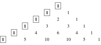
Example 2.2 (size of a simplex) As already mentioned, combinatorial topol-ogy derives its power from counting. Now that we have a finite description of a space, we can count easily. So, let’s use Figure 2.7 to count the number of faces of a simplex. For example, an edge has two vertices and an edge as its faces (recall that a simplex is a face of itself.) A tetrahedron has four vertices, six edges, four triangles, and a tetrahedron as faces. These counts are summa-rized in Table 2.1. What should the numbers be for a 4-simplex? The numbers in the table may look really familiar to you. If we add a 1 to the left of each
row, we getPascal’s triangle, as shown in Figure 2.9. Recall that Pascal’s
tri-angle encodes the binomial coefficients: the number of different combinations
oflobjects out ofkobjects ork
l
2.3 Simplicial Complexes 25
(a) The middle triangle shares an edge with the triangle on the left and a vertex with the triangle on the right.
(b) In the middle, the triangle is missing an edge. The simplices on the left and right intersect, but not along shared sim-plices.
[image:41.389.202.346.57.112.2]Fig. 2.8. A simplicial complex (a) and disallowed collections of simplices (b).
Table 2.1. Number of l-simplices in each k-simplex.
k/l 0 1 2 3
0 1 0 0 0
1 2 1 0 0
2 3 3 1 0
3 4 6 4 1
4 ? ? ? ?
k-simplex, anyl+1 of which defines anl-simplex. To make the relationship
complete, we define the empty set∅as the(−1)-simplex. This simplex is part
of every simplex and allows us to add a column of 1’s to the left side of Ta-ble 2.1 to get Pascal’s triangle. It also allows us to eliminate the underlined part of Definition 2.31, as the empty set of part of both simplices for nonin-tersecting simplices. To get the total size of a simplex, we sum each row of
1
1 1
1 2 1
1 3 3 1
1 4 6 4 1
[image:41.389.96.293.453.541.2]1 5 10 10 5 1
Pascal’s triangle. Ak-simplex haskl++11faces of dimensionland
k
∑
l=−1 k+
1
l+1
=2k+1
faces in total. A simplex, therefore, is a very large object. Mathematicians often do not find it appropriate for “computation,” when computation is being done by hand. Simplices are very uniform and simple in structure, however, and therefore provide an ideal computational gadget for computers.
2.3.2 Abstract Definition
The definition of a simplex uses geometry in a fundamental way. It might seem, therefore, that simplicial complexes have a geometric nature. It is possible to define simplicial complexes without using any geometry. We will present this definition next, as it displays the clear separation of topology and geometry that makes simplicial complexes attractive to us.
Definition 2.32 (abstract simplicial complex) Anabstract simplicial complex
is a setK, together with a collectionS of subsets ofK called(abstract)
sim-plicessuch that:
(a) For allv∈K,{v} ∈ S. We call the sets{v}theverticesofK.
(b) Ifτ⊆σ∈ S, thenτ∈ S.
When it is clear from the context whatS is, we refer toK as a complex. We
sayσis ak-simplexofdimension kif|σ|=k+1. Ifτ⊆σ,τis afaceofσand
σis acofaceofτ.
Note that the definition allows for∅ as a(−1)-simplex. We now relate this
abstract set-theoretic definition to the geometric one by extracting the combi-natorial structure of a simplicial complex.
Definition 2.33 (vertex scheme) LetKbe a simplicial complex with vertices
V and letKbe the collection of all subsets{v0,v1, . . . ,vk}ofV such that the
verticesv0,v1, . . . ,vkspan a simplex ofK. The collectionKis called thevertex
schemeofK.
The collectionKis an abstract simplicial complex. It allows us to compare
simplicial complexes easily, using isomorphisms.
2.3 Simplicial Complexes 27
with vertex setsV1,V2, respectively. AnisomorphismbetweenK1,K2is a
bi-jectionϕ:V1→V2, such that the sets inK1andK2are the same under the
renaming of the vertices byϕand its inverse.
Theorem 2.4 Every abstract complexSis isomorphic to the vertex scheme of some simplicial complex K. Two simplicial complexes are isomorphic iff their vertex schemes are isomorphic as abstract simplicial complexes.
The proof is in Munkres (1984).
Definition 2.35 (geometric realization) If the abstract simplicial complexS
is isomorphic with the vertex scheme of the simplicial complexK, we callK
ageometric realizationofS. It is uniquely determined up to an isomorphism, linear on the simplices.
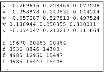
Having constructed a simplicial complex, we will divide it into topological and geometric components. The former will be an abstract simplicial com-plex, a purely combinatorial object that is easily stored and manipulated in a computer system. The latter is a map of the vertices of the complex into the space in which the complex is realized. Again, this map is finite, and it can be approximated in a computer using a floating point representation. This repre-sentation of a simplicial complex translates word for word into most common file formats for storing surfaces.
Example 2.3 (Wavefront Object File) One standard format is theObject File (OBJ)fromWavefront. This format first describes the map that places the
ver-tices inR3. A vertex with location(x,y,z)∈R3gets the line “vx y z” in the file.
After specifying the map, the format describes a simplicial complex by only listing its triangles, which are the principal simplices (see Definition 2.31). The vertices are numbered according to their order in the file and numbered from
1. A triangle with verticesv1,v2,v3is specified with line “fv1v2v3”. The
description in an OBJ file is often called a “triangle soup,” as the topology is specified implicitly and must be extracted.
2.3.3 Subcomplexes
Recall that a simplex is the power set of its simplices. Similarly, a natural view of a simplicial complex is that it is a special subset of the power set of all its
vertices. The subset isspecialbecause of the requirements in Definition 2.32.
v -0.269616 0.228466 0.077226 v -0.358878 0.240631 0.044214 v -0.657287 0.527813 0.497524 v 0.186944 0.256855 0.318011 v -0.074047 0.212217 0.111664 ...
f 19670 20463 20464 f 8936 8846 14300 f 4985 12950 15447 f 4985 15447 15448 ...
Fig. 2.10. Portions of an OBJ file specifying the surface of the Stanford Bunny.
a
d
e c
b
(a) A small complex
a b c
ac bc φ ab abc d e de cd
(b) Poset of the small complex, with prin-cipal simplices marked
φ φ
[image:44.389.111.278.45.162.2](c) An abstract poset: The “water level” of the poset is defined by principal simplices
Fig. 2.11. Poset view of a simplicial complex.
edge indicating a face-coface relationship. The marked principal simplices are
the “peaks” of the diagram. This diagram is, in fact, aposet.
Definition 2.36 (poset) LetSbe a finite set. A partial orderis a binary
re-lation≤onSthat is reflexive, antisymmetric, and transitive. That is for all
x,y,z∈S,
(a) x≤x,
(b) x≤yandy≤ximpliesx=y, and
(c) x≤yandy≤zimpliesx≤z.
A set with a partial order is apartially ordered set, orposetfor short.
2.3 Simplicial Complexes 29
Fig. 2.12. Closure, star, and link of simplices.
its waist because the number of possible simplicesn
k
is maximized fork≈
n/2. The principal simplices form a level beneath which all simplices must be
included. Therefore, we may recover a simplicial complex by simply storing its principal simplices, as in the case with triangulations in Example 2.3. This view also gives us intuition for extensions of concepts in point-set theory to simplicial complexes. A simplicial complex may be viewed as a closed set (it
isa closed point set, if it is geometrically realized).
Definition 2.37 (subcomplex, closure, link, star) Asubcomplexis a
simpli-cial complexL⊆K. The smallest subcomplex containing a subsetL⊆Kis ts
closure, ClL={τ∈K|τ≤σ∈L}. Thestar of Lcontains all of the cofaces
ofL, StL={σ∈K|σ≥τ∈L}. Thelink of Lis the boundary of its star,
LkL=Cl StL−St(ClL− {∅}).
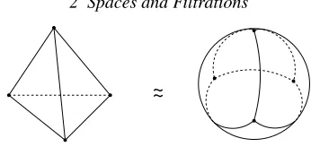
~
~
Fig. 2.13. The surface of a tetrahedron is a triangulation of a sphere, as its underlying space is homeomorphic to the sphere.
(b). The face relation is the partial order that defines “above” and “below.” Most of the time, the star of a set is an open set (viewed as a point set) and not a simplicial complex. The star corresponds to the notion of a neighborhood for a simplex and, like a neighborhood, it is open. The closure operation completes the boundary of a set as before, making the star a simplicial complex (b). The
link operation gives us the boundary. In our example, Cl{c,e} − ∅={c,e}, so
we remove the simplices from the light regions from those in the dark region
in (b) to get the link (c). Therefore, the link ofcandeis the edgeaband the
vertexd. Check on Figure 2.11(a) to see if this matches your intuition of what
a boundary should be.
2.3.4 Triangulations
We will use simplicial complexes to represent manifolds.
Definition 2.38 (underlying space) Theunderlying space|K|of a simplicial
complexKis|K|=∪σ∈Kσ.
Note that|K|is a topological space.
Definition 2.39 (triangulation) Atriangulationof a topological spaceXis a
simplicial complexKsuch that|K| ≈X.
For example, the boundary of a 3-simplex (tetrahedron) is homeomorphic to a sphere and is a triangulation of the sphere, as shown in Figure 2.13.
The term “triangulation” is used by different fields with different
mean-ings. For example, in computer graphics, the term most often refers to “triangle soup” descriptions of surfaces. The finite element community
of-ten refers to triangle soups as a mesh, and may allow other elements, such
as quadrangles, as basic building blocks. In areas, three-dimensional meshes
composed of tetrahedra are calledtetrahedralizations. Within topology, a
2.3 Simplicial Complexes 31
vertex a
edge
a b
c a b
tetrahedron a b
c
d
a [a, b]
triangle
[a, b, c] [a, b, c, d]
Fig. 2.14. k-simplices, 0≤k≤3. The orientation on the tetrahedron is shown on its faces.
2.3.5 Orientability
Our earlier definition of orientability (Definition 2.25) depended on differen-tiability. We now extend this definition to simplicial complexes, which are not smooth. This extension further affirms that orientability is a topological property not dependent on smoothness.
Definition 2.40 (orientation) LetKbe a simplicial complex. Anorientation
of ak-simplexσ∈K,σ={v0,v1, . . . ,vk}, vi∈K, is an equivalence class of
orderings of the vertices ofσ, where
(v0,v1, . . . ,vk)∼(vτ(0),vτ(1), . . . ,vτ(k)) (2.2)
are equivalent orderings if the parity of the permutationτis even. We denote
anoriented simplex, a simplex with an equivalence class of orderings, by[σ].
Note that the concept of orientation derives from that fact that permutations may be partitioned into two equivalence classes (if you have forgotten these concepts, you should review Definitions 2.4 and 2.15.) Orientations may be shown graphically using arrows, as shown in Figure 2.14. We may use oriented
simplices to define the concept of orientability to triangulatedd-manifolds.
Definition 2.41 (orientability) Twok-simplices sharing a(k−1)-faceσare
consistently orientedif they induce different orientations onσ. A triangulable
d-manifold isorientableif alld-simplices can be oriented consistently.
Other-wise, thed-manifold isnonorientable
But each triangle has two normals pointing in opposite directions. To get a correct rendering, we need the normals to be consistently oriented.
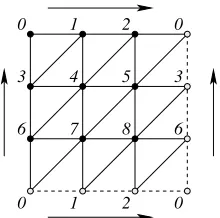
2.3.6 Filtrations and Signatures
All the spaces explored in this book will be simplicial complexes. We will explore them by building them incrementally, in such a way that all the subsets generated are also complexes.
Definition 2.42 (subcomplex) Asubcomplexof a simplicial complexKis a
simplicial complexL⊆K.
Definition 2.43 (filtration) Afiltrationof a complexKis a nested sequence
of subcomplexes,∅=K0⊆K1⊆K2⊆. . .⊆Km=K. We call a complexK
with a filtration afiltered complex.
Note that complexKi+1=Ki ∪˙ δi, whereδiis a set of simplices. The sets
δiprovide a partial order on the simplices of K. Most of the algorithms will
require a full ordering. One method to derive a full ordering is to sort eachδi
according to increasing dimension, breaking all remaining ties arbitrarily.
Definition 2.44 (filtration ordering) A filtration ordering of a simplicial
complexK is a full ordering of its simplices, such that each prefix of the
or-dering is a subcomplex.
We will index the simplices inK by their rank in a filtration ordering. We
may also build a filtration ofn+1 complexes from a filtration ordering ofn
simplices,σi,1≤i≤n, by adding one simplex at a time. That is,K0=∅and
fori>0,Ki={σj|j≤i}.
The primary output of algorithms in this book will be a signature function, associating a topologically significant value to each complex.
Definition 2.45 (signature) LetKibe a filtration ofm+1 complexes, and let
[m]denote the set{0,1,2, . . . ,m}of the complex indices. Asignature function
is a mapλ:[m]→R.
2.4 Alpha Shapes
2.4 Alpha Shapes 33
-1 0 1 2 3 4
0 2 4 6 8 10
Energy (kcal / mol)
Separation (Angstroms) Minimum Energy at 3.96 Angstroms
(a) The van der Waals force for two carbon atoms, as modeled by the Leonard-Jones potential function
[image:49.389.52.179.59.152.2](b) Gramicidin A, a protein, modeled as the union of spheres with van der Waals radii
Fig. 2.15. The van der Waals model for molecules.
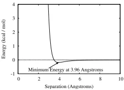
will present a method for generating such filtrations due to Edelsbrunner, Kirk-patrick, and Seidel (1983). The method has a natural affinity to space-filling
models of molecules. One such model is thevan der Waals model(Creighton,
1984). Thevan der Waals forceis a weak, but widespread force influencing
the structure of molecules. The force arises from the interaction between pairs of atoms. It is extremely repulsive in the short range and weakly attractive in the intermediate range, as shown in Figure 2.15(a) for two carbon atoms. Bi-ologists have captured the repulsive nature of this force by modeling atoms as spheres, as shown in Figure 2.15(b). The radii of atoms are defined to be half thevan der Waals contact distance, the distance at which the minimum energy is achieved. In reality, atoms should be viewed as balls with fuzzy bound-aries. Moreover, interactions of solvents with a molecule are often modeled by growing and shrinking of the balls. Generalizing this model, we could grow and shrink balls to capture all the possible shapes of a molecule. The alpha shapes model formalizes this idea. For a full mathematical exposition of the ideas discussed in this section, see Edelsbrunner (1995).
2.4.1 Dual Complex
We begin with the input to alpha shapes, a set of spherical balls.
Definition 2.46 (spherical balls) Aspherical balluˆ= (u,U2)∈R3×Ris
de-fined by its centeruand square radiusU2.
u
v
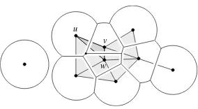
[image:50.389.123.265.43.121.2]w
Fig. 2.16. Union of nine disks, convex decomposition using Voronoï regions, and dual complex.
Definition 2.47 (weighted square distance) Theweighted square distanceof
a pointxfrom a ball ˆuisπuˆ(x) =x−u2−U2.
The weighted square distance of a pointxhas geometric meaning. It is the
square length of a line segment, tangent to the sphere, that hasxas one endpoint
and the tangent point as its other endpoint. A pointx∈R3belongs to