Simulation of Groundwater and Surface-Water Interaction and Effects of Pumping in a Complex Glacial-Sediment Aquifer, East Central Massachusetts

(1)

Prepared in cooperation with the Town of Framingham, Massachusetts

Simulation of Groundwater and Surface-Water

Interaction and Effects of Pumping in a Complex

Glacial-Sediment Aquifer, East Central Massachusetts

Land Surface

Bedrock Surface 100

300

200

-200 -100 0

Elevation, in feet above NGVD

West East

Layer 2 Layer 1

Layer 4 Layer 5

Sudbury River Lake Cochituate

Fines Fines _{Sand and gravel}

Fines

Bedrock and till

Layer 3

Sand and gravel Inactive model

Vertical exaggeration X 10

Scientific Investigations Report 2012–5172

(2)

(3)

Simulation of Groundwater and

Surface-Water Interaction and Effects of Pumping

in a Complex Glacial-Sediment Aquifer,

East Central Massachusetts

By Jack R. Eggleston, Carl S. Carlson, Gillian M. Fairchild, and Phillip J. Zarriello

Prepared in cooperation with the Town of Framingham, Massachusetts

Scientific Investigations Report 2012–5172

(4)

U.S. Department of the Interior

KEN SALAZAR, Secretary

U.S. Geological Survey

Marcia K. McNutt, Director

U.S. Geological Survey, Reston, Virginia: 2012

For more information on the USGS—the Federal source for science about the Earth, its natural and living resources, natural hazards, and the environment, visit http://www.usgs.gov or call 1–888–ASK–USGS. For an overview of USGS information products, including maps, imagery, and publications,

visit http://www.usgs.gov/pubprod

To order this and other USGS information products, visit http://store.usgs.gov

Any use of trade, firm, or product names is for descriptive purposes only and does not imply endorsement by the U.S. Government.

Although this information product, for the most part, is in the public domain, it also may contain copyrighted materials as noted in the text. Permission to reproduce copyrighted items must be secured from the copyright owner.

Suggested citation:

(5)

iii

Acknowledgments

A stakeholder interest group assembled for the study provided feedback and guided selection of model scenarios that were examined by the U.S. Geological Survey. Members of the stakeholder interest group include representatives from the towns of Framingham and Wayland, Massachusetts Water Resources Authority (MWRA), Massachusetts Department of Environmental Protection and Department of Conservation and Recreation, Massachusetts Executive Office of Environmental Affairs, U.S. Fish and Wildlife Service, U.S. Environmental Protection Agency, National Park Service, Organization for the Assabet River, Water Supply Citizens Advisory Committee, and SuAsCo (Sudbury-Assabet-Concord) Watershed Community Council. A separate technical advisory committee provided scientific oversight and technical guidance to the study and included the following non-USGS members: David Ahlfeld (University of Massachusetts), Grant Garven (Tufts University), and Daniel Nvule (MWRA). The authors gratefully acknowledge the guidance from the stakeholders’ interest group and the technical advisory committee.

(6)

(7)

v

Contents

Acknowledgments ...iii

Abstract ...1

Introduction...1

Purpose and Scope ...3

Study Area...3

Previous Investigations...3

Hydrogeology...4

Borehole Data...4

Geophysical Data ...4

Bedrock ...4

Glacial Sediment History ...6

Water Resources ...9

Surface-Water Features ...9

Groundwater Levels and Flow Paths ...13

Water Use ...17

Groundwater Flow Model ...18

Model Design...18

Discretization ...18

Model Boundaries ...21

Hydraulic Conductivity ...21

Storage Coefficients ...22

Streams...22

Recharge ...25

Pumping ...25

Model Calibration...25

Steady-State Calibration ...25

Transient Model Calibration ...29

Model Uncertainty and Sensitivity Analysis ...32

Model Limitations...36

Simulated Aquifer and Streamflow Response ...37

Steady-State Simulations ...38

Transient Model Simulations ...38

Evaluation of Pumping Strategies to Reduce Low-Flow Stresses ...40

Summary and Conclusions ...44

(8)

vi

Figures

1. Map showing glacial-sediment aquifer study area in east central Massachusetts ...2 2. Map showing well borings to bedrock, bedrock outcrops, passive seismic points,

and seismic lines used to develop the hydrogeologic framework and bedrock

surface topography, east central Massachusetts ...5 3. Graphs showing passive seismic A, response resonance frequency at known

bedrock depths and B, estimated and observed bedrock depths, east central

Massachusetts ...6 4. Map showing thickness of sediments above the bedrock surface in the study area,

east central Massachusetts ...7 5. Map showing locations of glacial-sediment deposits in the study area, east central

Massachusetts ...8 6. Hydrogeologic cross sections running north-south (A–A′ and B–B′) and

east-west (C–C′ and D–D′) through the study area, east central Massachusetts ...10 7. Map showing surface-water features and interpolated groundwater table

elevations in the study area, east central Massachusetts ...12 8. Photograph of Pod Meadow Pond showing open water along the southern shore in

February 2011, Framingham, Massachusetts ...14 9. Map showing active model area and boundary conditions, east central

Massachusetts ...19 10. Maps showing variability of hydraulic conductivity values of groundwater-model

layers 1–4 used in the calibrated model, east central Massachusetts ...20 11. Vertical cross sections of groundwater model layers and hydraulic conductivity

values running A, north-south and B, east-west, east central Massachusetts ...23 12. Maps showing model cells in layers 1–4 that dry in the calibrated steady-state

model, east central Massachusetts ...28 13. Graph showing observed and steady-state simulated groundwater levels, east

central Massachusetts ...29 14. Map showing simulated steady-state groundwater levels and errors, east central

Massachusetts ...30 15. Map showing wells used for transient model calibration of a glacial-sediment

aquifer model in east central Massachusetts ...31 16. Simulated and observed groundwater hydrographs, under current conditions and

no pumping at the Birch Road wells, east central Massachusetts ...33 17. Graph showing transient simulation of a 2006 aquifer test made with a daily time

step compared to groundwater observations, east central Massachusetts ...34 18. Map showing baseflow reduction (streamflow depletion) in stream-channel

segments in response to simulated pumping at the Birch Road wells at a constant rate of 4.9 cubic feet per second (3.17 million gallons per day), east central

Massachusetts ...39 19. Graph showing simulated transient monthly water budget under current average

monthly conditions (no pumping of Birch Road wells), east central Massachusetts ...40 20. Graph showing simulated streamflow response of the Sudbury River after 1 month

of pumping the Birch Road wells at 4.9 cubic feet per second (3.17 million gallons per day), east central Massachusetts ...41 21. Graph showing simulated monthly streamflows in the Sudbury River at the model

exit under five hypothetical pumping scenarios for the Birch Road wells, east

(9)

vii

22. Graph showing simulated streamflow along the Sudbury River for the month of September under average recharge rates and various pumping durations at the Birch Road wells, east central Massachusetts ...43 23. Graph showing percent reduction in Sudbury River simulated streamflow at the

model exit in response to pumping under average and dry recharge conditions, east central Massachusetts ...43

Tables

1. Discharge measurements at the outflows from Pod Meadow Pond and Dudley Pond, east central Massachusetts ...13 2. Borehole and groundwater observation wells used in the study, east central

Massachusetts ...15 3. Average groundwater withdrawal rates from Wayland production wells, 1996–2000

and 2002–2006, Wayland, Massachusetts ...17 4. Hydraulic conductivity of aquifer material and storage coefficients by layer in the

calibrated model, east central Massachusetts ...22 5. Stream segments and properties in the groundwater flow model, east central

Massachusetts ...24 6. Monthly recharge rates used in the transient groundwater flow model ...25 7. MODFLOW-NWT input file variable values for NWT package for transient

simulations of current conditions (scenario 4) ...26 8. Hydrologic characteristics and observed and simulated water levels of Pod

Meadow Pond, Dudley Pond, and Lake Cochituate, east central Massachusetts ...26 9. Simulated flows between Pod Meadow Pond, Dudley Pond, and Lake Cochituate

and the aquifer, east central Massachusetts ...27 10. Observed and simulated water levels and drawdowns from aquifer test of the

Birch Road wells, east central Massachusetts ...32 11. Model simulations used to determine sensitivity of induced recharge from

Lake Cochituate and pumping response times to hydraulic parameter values, east central Massachusetts ...35 12. Changes in induced recharge from Lake Cochituate and streamflow response

times resulting from changes in hydraulic parameter values, east central

Massachusetts ...35 13. Groundwater model scenarios used to evaluate the aquifer and streamflow

response to hypothetical withdrawals at the Birch Road wells, east central

Massachusetts ...37 14. Steady-state simulated water budgets with and without hypothetical Birch Road

well withdrawals, east central Massachusetts ...38 15. Simulated monthly flow in the Sudbury River under different hypothetical pumping

(10)

viii

Conversion Factors, Datum, and Abbreviations

Inch/Pound to SI

Multiply By To obtain

Length

foot (ft) 0.3048 meter (m)

mile (mi) 1.609 kilometer (km)

inch (in.) 2.54 centimeter (cm)

Area

square mile (mi2₎ _2.590 _{square kilometer (km}2₎

Flow rate

cubic foot per day (ft3_/d) _0.00001157 _{cubic foot per second (ft}3_/sec)

cubic foot per second (ft3_/s) _0.6463 _{million gallons per day (Mgal/d)}

million gallons per day (Mgal/d) 1.547 cubic foot per second (ft3_/s)

Vertical coordinate information is referenced to the North American Vertical Datum of 1988 (NAVD 88).

Horizontal coordinate information is referenced to the North American Datum of 1983 (NAD 83).

‘Elevation’, as used in this report, refers to distance above the vertical datum (NAVD 88).

Abbreviations

EIR Environmental Impact Report

MassDEP Massachusetts Department of Environmental Protection

MassDCR Massachusetts Department of Conservation and Recreation

MEPA Massachusetts Environmental Policy Act

MODFLOW-NWT MODular Groundwater FLOW Model with NeWTonian Solver

MWRA Massachusetts Water Resources Authority

NOAA National Oceanic and Atmospheric Administration

NPS National Park Service

NWIS National Water Information System

Ss Specific storage

Sy Specific yield

USFWS U.S. Fish and Wildlife Service

USEPA U.S. Environmental Protection Agency

(11)

Simulation of Groundwater and Surface-Water Interaction

and Effects of Pumping in a Complex Glacial-Sediment

Aquifer, East Central Massachusetts

By John R. Eggleston, Carl S. Carlson, Gillian M. Fairchild, and Phillip J. Zarriello

Abstract

The effects of groundwater pumping on surface-water features were evaluated by use of a numerical groundwater model developed for a complex glacial-sediment aquifer in northeastern Framingham, Massachusetts, and parts of surrounding towns. The aquifer is composed of sand, gravel, silt, and clay glacial-fill sediments up to 270 feet thick over an irregular fractured bedrock surface. Surface-water bodies, including Cochituate Brook, the Sudbury River, Lake Cochituate, Dudley Pond, and adjoining wetlands, are in hydraulic connection with the aquifer and can be affected by groundwater withdrawals.

Groundwater and surface-water interaction was simu-lated with MODFLOW-NWT under current conditions and a variety of hypothetical pumping conditions. Simulations of hypothetical pumping at reactivated water supply wells indicate that captured groundwater would decrease baseflow to the Sudbury River and induce recharge from Lake Cochituate. Under constant (steady-state) pumping, induced groundwater recharge from Lake Cochituate was equal to about 32 percent of the simulated pumping rate, and flow downstream in the Sudbury River decreased at the same rate as pumping. How -ever, surface water responded quickly to pumping stresses. When pumping was simulated for 1 month and then stopped, streamflow depletions decreased by about 80 percent within 2 months and by about 90 percent within about 4 months. The fast surface water response to groundwater pumping offers the potential to substantially reduce streamflow depletions during periods of low flow, which are of greatest concern to the eco -logical integrity of the river. Results indicate that streamflow depletion during September, typically the month of lowest flow, can be reduced by 29 percent by lowering the maxi -mum pumping rates to near zero during September. Lowering pumping rates for 3 months (July through September) reduces streamflow depletion during September by 79 percent as com -pared to constant pumping. These results demonstrate that a seasonal or streamflow-based groundwater pumping schedule can reduce the effects of pumping during periods of low flow.

Introduction

Glacial-sediment aquifers are an important source of water to communities in the northeastern United States. However, groundwater withdrawals from these aquifers are of growing concern because of their potential effects on surface-water resources, particularly streamflows. In the past, groundwater withdrawal limits were based on aquifer tests that determined the potential yield from wells with little regard to the effects of pumping on surface waters in hydraulic con-nection to the aquifer. More recent approaches to determining acceptable groundwater withdrawal rates include evaluating the long-term consequences of pumping on surface water resources and related ecosystems (Gleeson and others, 2011). The potential effects of groundwater withdrawals on surface-water features recently gained attention when the Town of Framingham (fig. 1) sought to reactivate production wells (the Birch Road wells) that previously provided a local water sup -ply from 1939 until about 1979. The wells were discontinued because of high iron and manganese concentrations and the availability of an alternative regional water supply.

In 2009, in accordance with the Massachusetts

(12)

2 Simulation of Groundwater and Surface-Water Interaction in a Glacial-Sediment Aquifer, Massachusetts

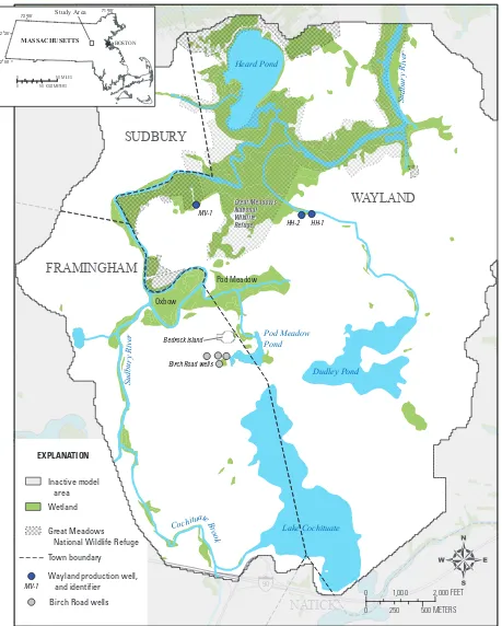
Figure 1. Glacial-sediment aquifer study area in east central Massachusetts.

90

Sudbury River Sudbury River

Sudbury River

CochituateBr_o o k

Dudley Pond

Lake Cochituate Heard Pond

Pod Meadow Pond Great Meadows National Wildlife Refuge Great Meadows National Wildlife Refuge

Bedrock island

WAYLAND

FRAMINGHAM

NATICK SUDBURY

WAYLAND

FRAMINGHAM

NATICK

SUDBURY

EXPLANATION

Wayland production well, and identifier

Inactive model area Wetland

Town boundary

Birch Road wells Great Meadows National Wildlife Refuge

Oxbow

Pod Meadow

Birch Road wells

Birch Road wells MV-1

HH-2 HH-1

MV-1

0 1,000

Base from U.S. Geological Survey and Massachusetts Geographic Information System data sources, Massachusetts State Plane Coordinate System, Mainland Zone

2,000 FEET

0 250 500 METERS

42o

00' 42o

30' 73o_00'

71o

00'

Study Area

MASSACHUSETTS BOSTON

(13)

Introduction 3

for migratory birds, fish, and other wildlife. In addition, environmental concerns were expressed in the MEPA review by state agencies, municipal agencies, and environmental interest groups, particularly about the effects of pumping on nearby Lake Cochituate, a state recreational resource.

The Sudbury River is considered stressed, particularly in its headwater reaches during low-flow periods, by develop -ment pressures and by numerous groundwater and surface-water withdrawals that affect streamflows (Zarriello and others, 2010). Concern about potential impacts of additional groundwater withdrawals on surface-water resources and aquatic ecology has led to a need for better understanding of the hydrologic system in the area of the proposed pump-ing. The purpose of this study by the U.S. Geological Survey (USGS), made in cooperation with the Town of Framing -ham, is to contribute to that understanding by presenting a compilation of existing and new hydrogeologic data and a new groundwater simulation model that was used to assess interactions between groundwater and surface water. The purpose of the groundwater model is to simulate present and hypothetical pumping conditions and to assess the potential to manage groundwater pumping to minimize its effect on nearby surface-water features. Hydraulic connections between surface water and aquifers are a growing concern across the country, and the techniques used in this study contribute to balancing the competing demands of water-supply needs with natural-resource protection, particularly in glacial-sediment aquifers in the northeastern United States.

Purpose and Scope

This report describes the development and calibration of a MODFLOW-NWT (Niswonger and others, 2011) ground -water model of the aquifer surrounding the Birch Road well site in Framingham, Massachusetts. The report also describes use of the model to simulate interaction between groundwater and surface-water features in the area under present conditions and scenarios of potential pumping from the Birch Road wells. The scenarios include alternative pumping rates and sched-ules that could reduce the effects of additional groundwater withdrawals on streams during low flows when the effects of withdrawals are most pronounced.

Study Area

The study area is 16 miles (mi) west of Boston in east central Massachusetts (fig. 1). The active groundwater model area covers about 6.1 square miles (mi2_{) surrounding the}

Birch Road wells in the towns of Framingham (1.7 mi2_),

Wayland (4.0 mi2_{), Sudbury (0.4 mi}2_{), and Natick (0.01 mi}2_).

The Sudbury River is the primary surface-water drainage feature, entering the study area from the southwest and discharging to the northeast. The Great Meadows National Wildlife Refuge (fig. 1) includes lands adjacent to the Sudbury River north of the oxbow and wetland areas in the northern

part of the study area, although most of the refuge is to the north of the study area. Lake Cochituate is the largest water body in the study area and has a 17.5 mi2_watershed

that is largely to the south and west of the study area. Lake Cochituate drains to the Sudbury River through the 1.4 mi long Cochituate Brook. Additional surface-water bodies include Dudley Pond, Pod Meadow Pond, and Heard Pond, which drain to the Sudbury River.

The aquifer is a complex mix of stratified glacially deposited sediments, including meltwater deltaic deposits and proglacial lake deposits that range in texture from clay to coarse gravel and boulders. Most of these deposits are medium to fine sands, which are the primary aquifer deposits.

Previous Investigations

The hydrology of the Lake Cochituate area was described by Gay (1985). Surficial geology of the study area was first described by Nelson (1974b, c) for the Framingham and Natick quadrangles and later updated by Stone and Stone (2006). Bedrock geology was described by Nelson (1974a, 1975) and updated by Zen and others (1983). Pond-aquifer interaction for the South Pond part of Lake Cochituate (south of the area shown in fig. 1) was investigated by Friesz and Church (2001). A hydrologic watershed model of the Sudbury and Assabet River basins was developed by Zarriello and oth -ers (2010) to simulate effects of water use and land use.

A variety of engineering consulting reports were published leading up to construction of the Massachusetts Water Resources Authority (MWRA) Metrowest water-supply tunnel that passes beneath the study area (Balsam Environmental Consultants 1986, 1987, and 1992). Seismic data were collected between 1989 and 1994 by GZA GeoEnvironmental, Inc. (1995). Aquifer characteristics, aquifer tests, and a one-layer groundwater model for the Birch Road well area were described by SEA Consultants, Inc., (1992, 2008) to evaluate reactivation of the Birch Road wells. Other observation wells and aquifer characteristics were described during investigations of nearby groundwater contamination (Sovereign Consulting, Inc., 2009; URS Corporation, 2003; IEP, Inc., 1983; Haley & Aldrich, 1996).

The Assabet-Sudbury River Basin study (Zarriello and others, 2010) includes end-member simulations of the effect of constant withdrawals from the Birch Road wells on river flow and Lake Cochituate water levels under assumed con -tribution or depletion of water from different surface-water sources. Hypothetical pumping was simulated at a constant rate of 6.65 cubic feet per second (ft3_{/s), with water coming}

(14)

4 Simulation of Groundwater and Surface-Water Interaction in a Glacial-Sediment Aquifer, Massachusetts

and flow could be mitigated if withdrawals were decreased at the appropriate times and by the appropriate amounts.” The current study looks at that possibility in greater detail.

Hydrogeology

Land surface elevations in the study area range from about 300 feet (ft) on the eastern margin to about 115 ft at the northeast outlet of the Sudbury River. Glacial-sediment deposits with complex stratification blanket a highly variable bedrock surface and fill a deep bedrock valley that underlies the north-south axis of Lake Cochituate. An understanding of the regional stratigraphic framework, geotechnical sediment classifications, and geologic depositional processes respon -sible for aquifer structure helps to appropriately represent the aquifer system in a groundwater flow model.

Borehole Data

Borehole data were compiled from consultant reports (Balsam Environmental Consultants, 1986, 1987, and 1992; GZA GeoEnvironmental, Inc., 1995; Haley & Aldrich, 1996; SEA Consultants, Inc., 1992, 2008; Sovereign Consulting, Inc., 2009; URS Corporation, 2003; and Bristol Engineering Advisors, Inc., 2011), USGS reports (Gay, 1981, 1985), and well construction reports kept at the USGS office in Northborough, Mass. Sedimentary logs and corresponding well construction records were available for 162 boreholes in the study area. These logs helped to establish details of the glacial sediment history and were used to define elevations and characteristics of hydrogeologic layers in the model.

Geophysical Data

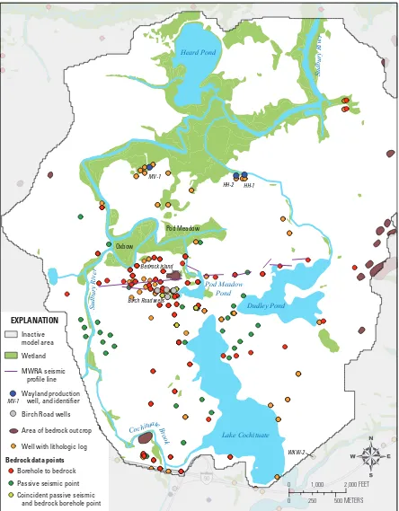
Geophysical data were compiled from previous studies and were collected during this study (fig. 2) to establish depth to bedrock. Seismic data were collected between 1989 and 1994 by the MWRA as part of a study for construction of a water-supply tunnel that passes beneath the study area (GZA GeoEnvironmental, Inc., 1995). Depths to bedrock data were determined by seismic refraction methods along the seismic lines shown in figure 2.

Passive seismic methods were used to measure depth to bedrock at 32 sites (fig. 2) where no borehole data were available and at 7 calibration sites where depths to bedrock were known. Passive seismic technology uses ambient ground vibrations caused by ocean waves, rainfall, wind, and anthro-pogenic activities to determine the thickness of unconsolidated sediments overlying bedrock (Ibs-von Seht and Wohlenberg, 1999; Lane and others, 2008). A three-component seismometer was used in this study to record the resonance frequency from ground vibrations, and a spectral analysis was made to obtain resonance frequencies related to the sediment thickness using equation 1.

Z

=

af

_r₀b_, ₍₁₎

where

Z is the depth to bedrock at a location, in feet;

f_r0 is the fundamental resonance frequency, in

hertz; and

a and b are constants determined by a nonlinear regression of data acquired at sites with known depths to bedrock.

Values for a (359.29) and b (-1.1979) were determined from the data collected at the seven control sites in the study area with known depths to bedrock (fig. 3A). The depths computed from equation 1 at the control sites generally better matched depths at higher resonance frequencies (shallower depths to bedrock) than at sites with lower resonance frequen -cies (deeper depths to bedrock). Depths to bedrock at the deeper control points in the study therefore were computed from calibrated coefficients (a = 297.24 and b = 1.00) deter -mined for Cape Cod (John Lane, U.S. Geological Survey, written commun., 2011), where depths to bedrock are gen -erally deeper and more closely matched depths than those computed from locally derived coefficients. Depths to bedrock were therefore determined at sites with resonance frequencies greater than about 2.5 hertz (depths less than about 120 ft) from locally derived coefficients and resonance frequencies less than about 2.5 hertz (depths greater than 120 ft) from coefficients derived for Cape Cod (fig. 3B). Of the 32 passive seismic sites without known bedrock depths, 19 had depths greater than 120 ft, and 14 had depths less than 120 ft.

Bedrock

(15)

Hydrogeology 5

Figure 2. Well borings to bedrock, bedrock outcrops, passive seismic points, and seismic lines used to develop the hydrogeologic framework and bedrock surface topography, east central Massachusetts.

90 Sudbury River Sudbury River

Sudbury River

Pod Meadow Pond

Dudley Pond

Lake Cochituate Heard Pond

Bedrock island

EXPLANATION

Wayland production well, and identifier

Bedrock data points Inactive model area

Borehole to bedrock

Passive seismic point

Coincident passive seismic and bedrock borehole point

MWRA seismic profile line

Well with lithologic log Wetland

Area of bedrock outcrop Birch Road wells

Oxbow

Pod Meadow

Birch Road wells

WKW-2 MV-1

HH-2 HH-1

MV-1

0 1,000

2,000 FEET

(16)

6 Simulation of Groundwater and Surface-Water Interaction in a Glacial-Sediment Aquifer, Massachusetts

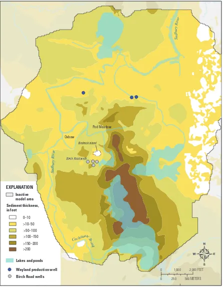
Elevation of the bedrock surface is highly variable with a deep bedrock valley following the north-south axis of Lake Cochituate. Bedrock surface elevations range from outcrops at about 300 ft on the east side of the study area to -118 ft at the bottom of the bedrock valley under Lake Cochituate (fig. 4). An isolated bedrock outcrop referred to as the “bedrock island” rises to an elevation of 165 ft just north of the Birch Road wells and drops steeply eastward to an elevation of

about -40 ft. The bedrock valley generally continues to rise to the north of the bedrock island, but few data are available to confirm the bedrock topography in this area. Bedrock topography likely determines groundwater flow patterns in the study area because bedrock is much less permeable than the overlying glacial deposits.

Nelson (1974a, 1975) and Goldsmith (1991) present two somewhat different interpretations of bedrock lithology in the study area. Nelson (1974a, 1975) indicated that bedrock underlying the study area is composed of three units: (1) the Cherry Brook Formation west of Lake Cochituate and west and north of Dudley Pond, (2) the Westboro Quartzite east of Dudley Pond, and (3) the Dedham Granodiorite east of Lake Cochituate. Goldsmith (1991) presented bedrock as two units: (1) quartzite and (2) metavolcanic rocks overlapping some -what with Nelson’s units. All the bedrock is thought to be relatively impermeable, although the upper bedrock surface is considered more fractured and permeable because of weather-ing and glacial movement. The upper bedrock in other parts of Massachusetts has been shown to have an active groundwater flow system that serves as a source of water to wells (Boutt and others, 2010; Mabee and others, 2002; and Hanson and Simcox, 1994). Groundwater flow through the bedrock of the study area was documented during construction of a water-supply tunnel at depths of 200–500 ft below land surface. Groundwater flow rates were weakly correlated with observed lineaments (Mabee and others, 2002), and therefore linea -ments were not represented in the model. In addition, ground -water levels in the glacial sediments and streamflow data do not indicate that the hydraulic properties of the bedrock affect shallow groundwater flow.

Glacial Sediment History

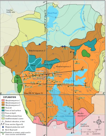
Overlying the bedrock in most of the study area are stratified glacial deposits laid down in the last stages of glacial Lake Charles during the retreat of the Wisconsin ice sheet (Clapp, 1904). A thin layer (generally 1–10 ft thick) of low-permeability glacial till lies immediately over bedrock in most areas. Thicker till deposits form several drumlin hills on the east and west sides of the study area (figs. 4, 5). Sedi -ments blanket till and bedrock over most of the study area and are interpreted as glacial meltwater deltaic deposits (Stone and Stone, 2006), similar to those recognized and mapped in many places in New England (Koteff and Pessl, 1981). As the glacier retreated to the north and northwest, it periodically paused and deposited gravel and sand at its terminus. Three glacial sediment morphosequences (fig. 5), identified by areas of stratified sediments contained between landforms and ice margins, have been documented in the study area (Stone and Stone, 2006; Janet Stone, U.S. Geological Survey, written commun., 2011). Generally, meltwater sediment deposits were finer grained where they settled in glacial Lake Charles away from the ice margin and coarser grained where they settled near the ice margin or mouth of the meltwater streams.

Figure 3. Passive seismic A, response resonance frequency at known bedrock depths and B, estimated and observed bedrock depths, east central Massachusetts.

y = 359.29x-1. 1979 R2_{= 0.99}

0

A. Resonance frequency

B. Estimated depth to bedrock

10 20 30

Resonance frequency, in Hertz

0 50 100 150 200 250

Estimated depth to bedrock, in feet

Depth to bedrock in b

o ri n g , i n fe e t

Depth to bedrock in b

o ri n g, i n fe e t Local

Bedrock depths based on horizontal to vertical spectral ratio (HVSR) for

(17)

Hydrogeology 7

Figure 4. Thickness of sediments above the bedrock surface in the study area, east central Massachusetts.

90

Sudbury River

S

u

d

b

u

r

y R

i ver

Bedrock island

EXPLANATION

Sediment thickness, in feet

0–10 >10–50 >50–100 >100–150 >150–200 >200

Inactive model area

Lakes and ponds

Oxbow

Pod Meadow

Birch Road wells

Wayland production well

Birch Road wells

0 1,000

2,000 FEET

(18)

8 Simulation of Groundwater and Surface-Water Interaction in a Glacial-Sediment Aquifer, Massachusetts

Figure 5. Locations of glacial-sediment deposits in the study area, east central Massachusetts.

90 Sudbury River

CochituateBr_o o k S u d b u r y R iver Dudley Pond Lake Cochituate Pod Meadow Pond Heard Pond -100 -50 -50 0 0 0 25 50 50 50 50 75 75 75 75 75 75 100 100 125 125 125 125 150 150 150 175 175 175 200 200 225 225 250 250 275 300 100 100 100 Bedrock island Bedrock island EXPLANATION Morphosequence 1 Undifferentiated fines Undifferentiated coarse Thick till

Fines at land surface Fines at depth

Morphosequence 3

Morphosequence 2

Morpho-sequence 1

Cross section (figure 6)

A A'

Bedrock elevation, in feet

50

Wayland production well

Borehole or seismic point used in cross section and identifier

F1W-49F1W-49 Inactive model area Morphosequence 2 Morphosequence 3 Inactive model area

Row 250, E-E’ (figure 11)

Column 125, A

’’-A

’’’ (figure 11)

E E' A'' A''' C C' D D' A' A B B'

Oxbow Pod Meadow

Birch Road wells

Birch Road well

F1W-60 Seismic-DSW WKB-51 WKW-117 WKW-27 Seismic-LA F1W-49 F1W-90 F1W-88 SEA-10 8-90 F1W-92 WKW-119 WKW-121 Seismic-DP-4 Seismic-LRCGR WKX-4 WKW-118 WKW-81 T-22C T-23 WKW-29 WKW-35 WKW-95 1-90 SEA-2 WKW-54 WKW-53 SEA-11 NS-21I NS-21H SEA-14 SEA-13 MW-5D MW-2D NS-21E NS-21J NS-21F T-19 T-18 Seismic-SLN Seismic-SSN F1W-60 Seismic-DSW WKB-51 WKW-117 WKW-27 Seismic-LA F1W-49 F1W-90 F1W-88 SEA-10 8-90 F1W-92 WKW-119 WKW-121 Seismic-DP-4 Seismic-LRCGR WKX-4 WKW-118 WKW-81 T-22C T-23 WKW-29 WKW-35 WKW-95 1-90 SEA-2 WKW-54 WKW-53 SEA-11 NS-21I NS-21H SEA-14 SEA-13 MW-5D MW-2D NS-21E NS-21J NS-21F T-19 T-18 Seismic-SLN Seismic-SSN 0 1,000

2,000 FEET

0 250 500 METERS

(19)

Water Resources 9

The sand and gravel deltaic deposits are interspersed with lower permeability fine-grained lacustrine deposits that are generally a mix of fine sands, silts, and clays (shown in light blue on fig. 5). Along geologic cross sections A–A′ and B–B′, extensive fine deposits are generally present below 140 ft in elevation in the southernmost parts of the sections and are mostly overlain by more permeable coarse-grain deposits except where they underlie Lake Cochituate (fig. 6A). Exten -sive fine deposits also are found in the northern part of the study area to the north of cross-section lines A–A′ and B–B′. Few borehole logs are available from this area to characterize these sediments, but those that do exist indicate that the fines consist of silty organic sediments, which may extend from the land surface to bedrock. The fine deposits in the middle part of the study area near the Birch Road wells are less extensive and slightly coarser (fine silts and silts) as indicated in cross-section lines C–C′ and D–D′ (fig. 6B). Contacts between sedi -ments were determined from well logs and from a theoretical understanding of the morphosequences in which they were deposited. However, the positions of boundaries are highly variable and poorly known in most locations.

Beneath kettle depressions such as Dudley Pond, Lake Cochituate, and Pod Meadow Pond, the sediments collapsed as the ice blocks beneath them melted. The high water-surface elevation of Dudley Pond (153 ft) relative to the elevations of nearby Lake Cochituate (138.5 ft) and Pod Meadow Pond (125.8 ft) is difficult to explain. Permeable sand and gravel deposits between the two sets of ponds should result in groundwater flow causing the level of Dudley Pond to drop closer to the level of Lake Cochituate. The reason these ponds can maintain such a high hydraulic gradient may lie at the bot-tom of the ponds. Sediment cores collected as part of an eutro -phication study of Dudley Pond by the Town of Wayland (IEP, Inc., 1983) indicated a layer of bottom muck sediments up to 14 ft thick. This muck layer, referred to as gyttja, is partially decayed organic material that settles out of the water column though time and has a black gel-like consistency. These depos -its are an impediment to seepage losses from the pond to the aquifer and a likely explanation for why Dudley Pond exists and why the surface level does not substantially drop during the late summer when inflows to the pond are typically small. Similar deposits are believed to underlie parts of northern Lake Cochituate (dark blue in sections B–B′, C–C′, and D–D′, figs. 6A and B) as evidenced by up to 12 ft of gyttja depos -its determined from ground-penetrating radar surveys of the South Pond of Lake Cochituate (Friesz and Church, 2001).

Water Resources

Surface water generally is in hydraulic connection with groundwater in the study area. Both surface water and ground-water are supplied by abundant precipitation, with average annual precipitation in 2004–09 measuring about 50 inches (in) at nearby Natick, Mass. (National Oceanic and Atmo -spheric Administration (NOAA) station USC00195175).

Surface-Water Features

The major surface-water features in the study area include the Sudbury River to the west and north, the northern -most pond of Lake Cochituate to the south, Cochituate Brook to the southwest, Dudley Pond to the east, and Pod Meadow Pond (fig. 7). The shallow and permeable aquifer system is generally in close hydraulic connection with the abundant surface-water features in the study area, but the connection may be locally constrained by gyttja deposits in lakes and ponds as previously described.

Lake Cochituate consists of four ponds (only the north -ernmost is shown in fig. 7) connected by shallow, narrow waterways that form a relatively long south-north trend-ing lake. Total drainage area at the lake outlet is 17.5 mi2_.

The lake is a series of kettle ponds formed following the last glacial retreat. Of these four connected ponds, only the northernmost pond—hereafter called “Lake Cochituate”—is in the study area. This part of the lake has a 0.31 mi2_surface

area and drains to the westward-flowing Cochituate Brook that connects to the northeastward-flowing Sudbury River. Streamflow in Cochituate Brook (fig. 7) was monitored by the USGS (01098500) from October 1977 to June 1979 and from August 2010 through June 2012. Daily mean flow for this entire period was 34.9 ft3_{/s. Lake Cochituate stage has}

been continuously monitored by the USGS (01098499) since August 2010, during which time the lake level varied by 2.1 ft through December 2011 and was lowest during parts of the summer when levels dropped below the crest of the outlet spillway. Flow and stage data collected by the USGS are maintained in the National Water Information System (NWIS), which is available at http://waterdata.usgs.gov/nwis.

Other ponds in the study area include Dudley Pond northeast of Lake Cochituate, Pod Meadow Pond north of Lake Cochituate, and Heard Pond in the north-central part of the study area (fig. 7). Heard Pond was not explicitly modeled because of its distance from the Birch Road wells and location on the opposite side of the Sudbury River. Dudley Pond, also a kettle pond, has a surface area of 0.14 mi2_{and a total}

drain-age area of 0.58 mi2_{measured at its outlet. Pod Meadow Pond}

has a surface area of 0.01 mi2 _{and a drainage area of 0.23 mi}2_. Early topographic maps show Pod Meadow Pond as a wetland that was likely modified by sand and gravel excavations in the early to mid-20th century.

Outflows from Pod Meadow Pond and Dudley Pond (fig. 7) were measured monthly starting in March 2011 to provide data for groundwater model calibration. The quality of streamflow measurement data was generally considered good to fair, but was poor (as defined by Kennedy, 1983) at the lowest flows because of low stream depth and velocity. Drainage areas at the outflow measurement sites to Pod Meadow Pond and Dudley Pond are 0.23 and 0.58 mi2_,

(20)

10

Simulation of Groundwater and Surface-W

ater Interaction in a Glacial-Sediment Aquifer

, Massachusetts

Figure 6. Hydrogeologic cross sections running north-south (A–A′ and B–B′) andeast-west (C–C′ and D–D′) through the study area, east central Massachusetts.

200 220 80 180 160 140 120 100 60 40 20 -20 0 Massachusetts Turnpike Gyttja Gyttja Lake Cochituate Dudley Pond B' B South North WKB-51 WKW -117 WKW -27 WKW -118 WKX-4 T-22C WKW -35 WKW -95, projected Bedrock Sand and gravel

Sand Fines Sand Fines Till 4,000 2,000

0 6,000 8,000 10,000 12,000 14,000

Distance, in feet

Elevation, in feet above NAVD 88

A' A

Cochituate Brook

Bedrock

Boundaries between units are mostly uncertain Till

Lake Cochituate level

Sand and gravel

Fine to very fine sand or silt

Sand Sand Seismic-LA Seismic-DSW F1W -60 F1W -49 F1W -90 F1W -88 SEA-10 8-90 1-90 SEA-2 200 220 80 180 160 140 120 100 60 40 20 0

0 1,000 2,000 3,000 4,000 5,000 6,000 7,000 8,000

Distance, in feet

South North

Fines

Boundaries between most contacts are uncertain EXPLANATION

Fine to very fine sand or silt Sand

Fines (silt and clay)

Sand and gravel

Till Bedrock Kettle depression

Vertical exaggeration X 20 Vertical exaggeration X 20

Gyttja (organic muck)

90

Geologic interpretation assisted by Janet A. Stone, 2011

SECTION D–D’ SECTION C–C’

(21)

Figure 6. Hydrogeologic cross sections running north-south (A–A′ and B–B′) andeast-west (C–C′ and D–D′) through the study area, east central Massachusetts.—Continued

Screened interval of SEA test wells, 800 feet to north

Artificial fill 0 200 80 180 160 140 120 100 60 40 20 -20 -40 -60 220 240 -80 200 80 180 160 140 120 100 60 40 20 0 -20 -40 -60 220 Dudley Pond

Birch Road wells screened interval 400 feet to south

Sudbury River Pod Meadow Pond C' C West East D' D West East T-18 T-19 MW -5D MW -2D NS-21F NS-21H Seismic-SSN Seismic-SLN NS-21I SEA-11 SEA-10 F1W -92 WKW -119 WKW -121 Seismic-LRCGR Seismic-DP4 NS-21J SEA-13 SEA-14 WKW -54 T-22C T-23 WKW -53 NS-21E

Lake Cochituate level

Sudbury River Lake Cochituate Dudley Pond WKW -81

Boundaries between units are mostly uncertain

Bedrock

Till

Sand and gravel

Sand

Bedrock

Till Sand

Sand and gravel

Sand

Gyttja

Gyttja Gyttja

Gyttja

0 1,000 2,000 3,000 4,000 5,000 6,000 7,000 8,000 9,000

0 1,000 2,000 3,000 4,000 5,000 6,000 7,000 8,000 9,000 10,000

Distance, in feet

EXPLANATION

Sand

Sand and gravel

Till

Bedrock

Gyttja (organic muck)

Kettle depression

Vertical exaggeration X 20

Geologic interpretation assisted by Janet A. Stone, 2011

(22)

12 Simulation of Groundwater and Surface-Water Interaction in a Glacial-Sediment Aquifer, Massachusetts

Figure 7. Surface-water features and interpolated groundwater table elevations in the study area, east central Massachusetts.

120

120 120

130

130 130

130

140

150

160

160 160

90

Sudbury River Sudbury River

S u

d

b

u

r

y

R

iv

er

Heard Pond

Dudley Pond

Lake Cochituate Pod Meadow Pond Bedrock island

Bedrock island

EXPLANATION

Groundwater-table elevation (approximate) General direction of groundwater flow Wetland

120

Observation well used to draw water table, and identifier

Wayland production well, and identifier USGS streamgage

and number Inactive model area

Birch Road wells

Pod Meadow Pond outflow

01098500 01098500

USGS partial-record streamgage

01098530

Dudley Pond outflow

WKW-119

F1W-84 MW-8

MW-1

F1W-84

Oxbow

Pod Meadow

Birch Road wells

MV-1

HH-2 HH-1

0 1,000

2,000 FEET

0 250 500 METERS

(23)

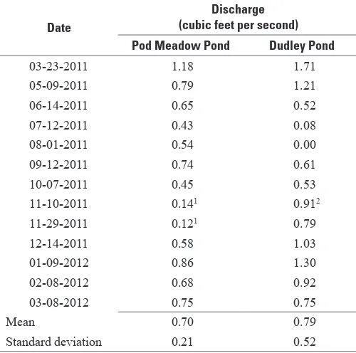
pool upstream of the measurement site. Discharge from Pod Meadow Pond also was relatively consistent, ranging from 0.43 to 1.18 ft3_{/s, compared to the outflow from Dudley Pond,}

which ranged from 0 to 1.71 ft3_{/s. The relatively high and}

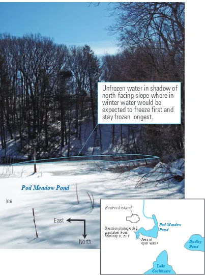
consistent outflow from Pod Meadow Pond, which has a small contributing area relative to Dudley Pond, suggests a larger groundwater discharge to Pod Meadow Pond than to Dudley Pond. This higher outflow is also evident from anecdotal reports that the southwestern part of Pod Meadow Pond does not freeze, which was confirmed during site visits in the winter of 2010–11 (fig. 8) when both Lake Cochituate and Dudley Pond were completely frozen and part of Pod Meadow Pond was not, indicating discharge of relatively warm groundwater. Factors that could contribute to the groundwater discharge at Pod Meadow Pond include its low topographic position, removal of surface material and lowered topography as a result of past mining activities, occurrence of high permeability sand and gravel, proximity to Lake Cochituate and related steep hydraulic gradient to the lake, increasing bedrock elevation forcing groundwater flow upward, and the pond’s position just north of the edge of the extensive layer of low-permeability fine-grained sediments.

Extensive wetlands exist adjacent to the Sudbury River and other streams in the northern part of the study area. Pod

Meadow Pond drains north into the Pod Meadow wetland, which then drains into the oxbow on the Sudbury River. Just north of the oxbow, the Sudbury River meanders through extensive wetlands that are part of the Great Meadows National Wildlife Refuge (fig. 1).

The Sudbury River flows from the southwest toward the northeast through the study area and is the primary drainage feature that likely receives all groundwater discharge from the study area aquifer, either directly or indirectly from numerous tributaries. The drainage area of the Sudbury River is about 85 mi2_{at its entrance to the study area and about}

111 mi2_{at its exit from the study area. Groundwater levels} indicate that there is little or no groundwater crossing beneath the river. Flow in the Sudbury River near the southwestern boundary of the study area has been continuously monitored at Saxonville (01098530) since October 1979. Mean daily flow at Saxonville from October 1979 through September 2009 was 205 ft3_{/s with monthly mean flows ranging from 71 ft}3_{/s in}

September to 384 ft3_{/s in April.}

Groundwater Levels and Flow Paths

Groundwater level measurements collected in and near the study area for a variety of purposes were compiled for this study. Groundwater levels were obtained from NWIS or compiled from previous site investigations (Balsam, 1987, 1992; SEA, 1992, 2008). Additional groundwater observations were also made during this study (Peter Newton, Bristol Engineering Advisors, Inc., written commun., 2011). The complete set of groundwater level observations (table 2) spans the period from 1931 through 2011. Water levels from individual observation wells span shorter periods, were obtained over a wide range of hydroclimatic conditions, and may not represent the long-term average.

Water levels from observation wells and surface eleva -tions of water bodies were used to develop a water-table map (fig. 7), which was manually interpolated and contoured. The water-table map indicates that regional groundwater flow is towards the Sudbury River. Groundwater discharges to the eastern boundary of Lake Cochituate from both the deep and shallow aquifer, but along the western lake boundary, ground -water flow in the shallow aquifer is towards the lake while groundwater flow in the deeper aquifer is away from the lake towards the Sudbury River.To the west of Lake Cochituate, water levels in shallow wells have been measured as much as 20 ft higher than water levels in deep wells. The low-permeability lacustrine deposits in this area may cause locally perched water table conditions, hydraulically separating the upper and lower parts of the aquifer (fig. 6A). Groundwater levels from vertically paired wells in other parts of the study area (not shown in fig. 7) indicate little difference between shallow and deep parts of the aquifer, indicating that the aquifer is unconfined, and that deep and shallow levels of the aquifer are probably hydraulically well connected.

Table 1. Discharge measurements at the outflows from Pod Meadow Pond and Dudley Pond, east central Massachusetts.

Date

Discharge (cubic feet per second)

Pod Meadow Pond Dudley Pond

03-23-2011 1.18 1.71

05-09-2011 0.79 1.21

06-14-2011 0.65 0.52

07-12-2011 0.43 0.08

08-01-2011 0.54 0.00

09-12-2011 0.74 0.61

10-07-2011 0.45 0.53

11-10-2011 0.141 _0.912

11-29-2011 0.121 _0.79

12-14-2011 0.58 1.03

01-09-2012 0.86 1.30

02-08-2012 0.68 0.92

03-08-2012 0.75 0.75

Mean 0.70 0.79

Standard deviation 0.21 0.52

1_{Discharge affected by beaver dam that was impounding water; values} excluded from mean and standard deviation.

(24)

Figure 8. Pod Meadow Pond showing open water along the southern shore in February 2011, Framingham, Massachusetts.

North

East

Unfrozen water in shadow of

north-facing slope where in

winter water would be

expected to freeze first and

stay frozen longest.

Ice

Pod Meadow Pond

Dudley Pond

Bedrock island

Direction photograph was taken from, February 11, 2011

Lake Cochituate

(25)

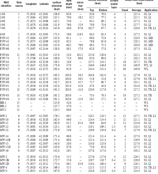
Table 2. Borehole and groundwater observation wells used in the study, east central Massachusetts.—Continued

[Well locations shown in figures 7 and 15; Elevation in North American Vertical Datum 1988; SS, used to calibrate steady-state model; TR, used to calibrate tran

-sient model; LI, used to determine lithology; WL, water level(s) used to develop model; WS, water-supply well; --, no data available. Data sources are: 1, SEA Consultants, Inc. (1992); 2, SEA Consultants, Inc., (2008); 3, Gay (1985); 4, Gay (1981); 5, Balsam (1987, volume I); 6, Balsam (1987, volume II); 7, Balsam (1992, volume I); 8, Balsam (1992, volume II); 9, Sovereign Consulting, Inc. (2009); 11, U.S. Geological Survey files in Northborough, Mass. (accessed 2011); 13, National Water Information System (NWIS) online at http://waterdata.usgs.gov/nwis; 15, Wayland Wellhead Protection Committee and Bruce W. Young

(2011)]

Well identifier

Data

source Longitude Latitude

Land surface elevation

(feet)

Hole depth

(feet)

Bedrock

eleva-tion (feet)

Screen elevation (feet)

Screen model layer

Water-level observations (feet)

Top Bottom Count Average Application

1-90 1 -71.3858 42.3301 136.0 63.0 -- 83.0 78.0 4 1 125.4 SS, LI

2-90 1 -71.3864 42.3305 135.5 79.0 56.5 82.5 77.5 4 1 125.5 SS, LI

3-90 1 -71.3872 42.3306 145.1 74.0 -- 94.1 89.1 4 4 127.3 SS, LI

5-90 1 -71.3878 42.3306 131.9 76.0 55.9 78.9 73.9 4 4 127.7 SS, LI

7-90 1 -71.3876 42.3324 145.6 48.0 97.6 102.7 97.7 4 4 120.0 SS, TR, LI

8-90 1 -71.3858 42.3293 172.3 56.0 116.3 88.3 83.3 4 4 127.2 SS, LI

F1W-41 3 -71.3864 42.3297 135.0 61.1 -- 90.0 72.0 4 1 128.9 SS, MD

F1W-42 3 -71.3875 42.3306 142.0 62.3 -- 76.6 61.6 4 1 128.2 SS, MD

F1W-43 3 -71.3886 42.3303 135.0 60.2 76.0 89.3 71.3 4 1 130.9 SS, MD

F1W-60 4 -71.3867 42.3144 138.0 80.1 57.8 62.8 57.8 4 1 137.3 SS, LI

F1W-64 11 -71.3961 42.3342 125.0 23.8 101.2 125.0 120.0 1 1 122.1 SS, LI

F1W-74 5 -71.3789 42.3144 140.0 71.0 69.0 95.0 90.0 4 1 138.2 SS, LI

F1W-84 3 -71.3856 42.3256 139.5 18.0 -- 127.5 124.5 2 16 137.5 SS, TR

F1W-85 3 -71.3847 42.3183 173.0 37.0 -- 149.0 146.0 2 19 149.9 WL, LI

F1W-87 3 -71.3858 42.3272 193.4 65.0 -- 134.4 131.4 2 49 149.6 WL

F1W-88 3 -71.3858 42.3272 193.3 163.0 30.3 104.8 101.8 4 11 127.6 SS, LI

F1W-89 3 -71.3858 42.3272 193.3 163.0 30.3 55.6 52.6 4 8 127.6 SS, TR, LI

F1W-90 3 -71.3856 42.3256 142.7 101.0 45.7 71.7 68.7 4 8 133.1 SS, LI

F1W-91 3 -71.3856 42.3256 142.8 101.0 45.8 47.8 44.8 4 8 134.0 SS, TR, LI

F1W-92 13 -71.3889 42.3142 191.2 203.0 -11.8 120.0 117.0 2 9 127.2 SS, TR, LI

F1W-93 13 -71.3833 42.3289 191.2 203.0 -- 73.3 70.3 4 10 127.2 SS, TR

F1W-94 4 -71.3833 42.3289 191.2 203.0 -11.8 20.5 17.5 4 9 127.1 SS, LI

HH-1 15 -- -- 125.9 42.0 -- -- -- 4 -- -- WS

HH-2 15 -- -- 125.7 47.0 -- -- -- 4 -- -- WS

MV-1 15 -- -- 124.5 80.0 -- -- -- 4 -- -- WS

MW-1 6 -71.3907 42.3305 176.5 60.5 -- 128.5 118.5 4 12 127.1 SS, TR, LI

MW-10 6 -71.3916 42.3320 162.4 49.0 -- 124.4 114.4 2 11 121.1 SS, LI

MW-11 6 -71.3916 42.3320 162.9 81.5 81.4 89.9 84.9 4 12 124.6 SS, LI

MW-12 6 -71.3901 42.3334 123.1 16.5 -- 119.1 109.1 1-2 9 118.3 SS, LI

MW-13 6 -71.3898 42.3310 171.6 54.0 -- 129.6 119.6 3-4 7 127.6 SS, TR, LI

MW-14 6 -71.3898 42.3309 171.4 60.0 -- 121.4 111.4 4 4 127.8 SS, LI

MW-14R 6 -71.3898 42.3309 171.4 60.0 -- 121.4 111.4 4 2 126.9 SS, LI

MW-15 8 -71.3893 42.3307 143.0 20.0 -- 133.0 123.0 2 2 127.0 SS, LI

MW-15D 8 -71.3892 42.3307 143.0 87.0 -- 75.0 65.0 4 2 127.3 SS, LI

MW-16 8 -71.3887 42.3312 142.8 26.5 -- 137.8 117.8 2 2 130.2 SS, LI

MW-2 6 -71.3918 42.3312 172.6 55.5 -- 127.6 117.6 4 12 126.5 SS, LI

MW-2B 6 -71.3918 42.3312 172.7 55.0 -- 129.7 119.7 3-4 11 126.9 SS, LI

MW-2D 6 -71.3917 42.3312 172.4 86.5 85.9 110.4 100.4 4 6 126.1 SS, LI

MW-3 6 -71.3920 42.3314 169.3 55.5 -- 125.3 115.3 4 12 128.2 SS, TR, LI

(26)

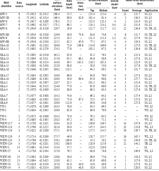
Table 2. Borehole and groundwater observation wells used in the study, east central Massachusetts.—Continued

[Well locations shown in figures 7 and 15; Elevation in North American Vertical Datum 1988; SS, used to calibrate steady-state model; TR, used to calibrate tran

-sient model; LI, used to determine lithology; WL, water level(s) used to develop model; WS, water-supply well; --, no data available. Data sources are: 1, SEA Consultants, Inc. (1992); 2, SEA Consultants, Inc., (2008); 3, Gay (1985); 4, Gay (1981); 5, Balsam (1987, volume I); 6, Balsam (1987, volume II); 7, Balsam (1992, volume I); 8, Balsam (1992, volume II); 9, Sovereign Consulting, Inc. (2009); 11, U.S. Geological Survey files in Northborough, Mass. (accessed 2011); 13, National Water Information System (NWIS) online at http://waterdata.usgs.gov/nwis; 15, Wayland Wellhead Protection Committee and Bruce W. Young

(2011)]

Well identifier

Data

source Longitude Latitude

Land surface elevation

(feet)

Hole depth (feet)

Bedrock

eleva-tion (feet)

Screen elevation (feet)

Screen model layer

Water-level observations (feet)

Top Bottom Count Average Application

MW-5 6 -71.3913 42.3315 169.4 55.5 -- 125.4 115.4 4 12 125.7 SS, LI

MW-5D 8 -71.3912 42.3314 169.4 89.0 82.9 101.4 91.4 4 2 126.2 SS, LI

MW-6 6 -71.3917 42.3299 176.3 55.5 -- 132.3 122.3 4 2 131.9 SS, LI

MW-7 6 -71.3901 42.3317 173.1 60.5 -- 124.1 114.1 3-4 11 131.0 SS, LI

MW-8 6 -71.3919 42.3326 129.7 19.0 -- 121.7 111.7 1-2 12 120.6 SS, TR, LI

MW-8D 6 -71.3919 42.3326 129.6 56.0 73.6 84.6 74.6 4 6 121.7 SS, TR, LI

MW-9 6 -71.3910 42.3330 125.3 18.5 -- 121.3 111.3 1-2 12 117.9 SS, LI

MW-9D 6 -71.3910 42.3330 125.5 62.5 65.0 77.5 67.5 4 4 119.8 SS, LI

SEA-10 2 -71.3861 42.3282 180.6 72.0 108.6 114.6 109.6 4 3 127.9 SS, TR, LI

SEA-11 2 -71.3892 42.3279 174.2 77.0 -- 102.2 97.2 4 3 129.6 SS, TR, LI

SEA-12 2 -71.3893 42.3316 161.2 85.0 -- 81.2 76.2 4 3 121.8 SS, LI

SEA-13 2 -71.3894 42.3311 155.6 95.5 60.1 93.6 88.6 4 3 127.8 SS, LI

SEA-14 2 -71.3880 42.3314 144.8 39.5 105.3 110.3 105.3 4 3 121.9 SS, LI

SEA-15 2 -71.3888 42.3338 122.0 98.0 -- 58.0 53.0 4 3 117.6 SS, TR, LI

SEA-16 2 -71.3846 42.3265 186.2 123.5 -- 94.2 89.2 4 3 131.7 SS, LI

SEA-17 2 -71.3884 42.3305 139.0 60.0 -- 84.0 79.0 4 3 127.8 SS, LI

SEA-18 2 -71.3869 42.3291 149.0 59.0 90.0 95.0 90.0 4 3 127.7 SS, LI

SEA-2 2 -71.3859 42.3307 128.7 32.5 -- 101.2 96.2 4 3 125.6 SS, LI

SEA-3 2 -71.3844 42.3313 124.0 77.0 -- 65.0 60.0 4 3 122.4 SS, TR, LI

SEA-4 2 -71.3870 42.3300 143.3 80.0 -- 68.3 63.3 4 3 127.6 SS, TR, LI

SEA-7 2 -71.3877 42.3308 134.2 74.0 -- 69.2 64.2 4 3 127.9 SS, LI

SEA-8 2 -71.3863 42.3305 138.3 71.0 67.3 72.3 67.3 4 3 127.0 SS, LI

SEA-9 2 -71.3877 42.3301 139.0 112.0 -- 39.0 34.0 4 3 127.8 SS, LI

TW-1 2 -71.3870 42.3299 143.3 78.0 -- 84.3 69.3 4 -- -- WS, LI

TW-2 2 -71.3884 42.3305 139.0 61.0 -- 89.0 79.0 4 -- -- WS, LI

TW-3 2 -71.3872 42.3306 134.2 73.0 -- 79.2 64.2 4 -- -- WS, LI

TW-4 2 -71.3863 42.3305 138.3 67.2 -- 86.1 71.1 4 -- -- WS, LI

WKW-117 4 -71.3730 42.3181 138.4 32.0 -- 136.9 136.7 1 14 137.6 SS, LI

WKW-118 3 -71.3700 42.3225 181.0 38.0 -- 147.5 144.5 3 23 153.6 WL, LI

WKW-119 3 -71.3822 42.3286 175.1 65.0 -- 117.5 114.5 2 16 129.7 SS, TR, LI

WKW-120 3 -71.3714 42.3200 175.7 49.0 -- 158.7 155.7 -- 16 165.5 WL, LI

WKW-123 3 -71.3786 42.3281 150.2 100.0 -- 53.2 50.2 4 12 138.9 SS, TR, LI

WKW-124 3 -71.3786 42.3281 150.2 100.0 -- 128.9 125.9 2 12 144.2 TR, LI

WKW-2 13 -71.3681 42.3144 153.8 37.5 -- 122.8 120.8 -- -- -- LI

WKW-27 4 -71.3736 42.3194 155.0 76.5 -- 88.6 78.6 -- 1 149.0 WL, LI

WKW-30 13 -71.3883 42.3389 120.0 50.0 -- 80.0 75.0 4 1 118.8 SS, LI

WKW-52 13 -71.3894 42.3425 118.0 61.5 -- 65.0 60.0 4 1 117.0 SS, LI

WKW-53 11 -71.3819 42.3319 135.0 91.0 44.0 54.0 49.0 2 1 127.0 SS, LI

(27)

Subsets of the groundwater-level data were used in model calibration. Groundwater level observations from 65 wells were used in calibrating the steady-state groundwater model. Twelve of these 65 wells have a single measurement, and the remaining have a median of 3 measurements spanning a median period of 30 days. Wells with more than 3 observations had a median difference between the minimum and maximum observations of 2.2 ft. Groundwater level observations from 13 wells were used in calibrating the transient groundwater model. A set of groundwater level observations collected during a 2006 aquifer test (SEA Consultants, Inc., 2008) also was used for calibrating both the steady-state and transient models. Many observation wells were excluded from the model calibration because of uncertainty about well locations, land-surface elevations, well depths, or screened intervals.

Water Use

A permit from the Massachusetts Department of Environmental Protection (MassDEP) is required for all public water-supply withdrawals and for large nonpotable-water withdrawals (industrial and agricultural, for example). The Town of Wayland has the only permitted groundwater withdrawals in the study area and pumps water from three production wells north of the Birch Road well site near the Sudbury River (MassDEP numbers 3315000–03G; –04G; –05G, labeled HH-1, HH-2, and MV-1, respectively, in fig. 7). These three wells have an average annual combined withdrawal of 1.40 ft3_{/s, equal to 0.90 million gallons per day}

(Mgal/d). Monthly average withdrawals peak in July with seasonal high withdrawals from May through September that are 9 to 34 percent greater than the annual average (table 3) based on records from 1996–2000 and 2002–2006.

From 1939 to 1979, the Town of Framingham oper -ated wells at the Birch Road site for municipal water supply (fig. 7). The production wells consisted of a cluster of three wells about 1,400 ft north of Lake Cochituate and about 600 ft southeast of the Sudbury River. The wells had a combined pumping capacity of 5.3 ft3_{/s (3.5 Mgal/d) but were likely}

pumped at a rate closer to 4.9 ft3_{/s (SEA Consultants, Inc.,}

1992). The wells were operated intermittently during the mid- to late 1970s because of high iron and manganese concentra -tions, and their use was eventually discontinued in 1979. The town currently obtains all of its water from MWRA from sources outside of the study area. Four large-diameter wells (Birch Road wells, fig. 7) that were installed for aquifer tests in 2005 may become the supply wells for future withdrawals and are treated as such in this study.

Lake Cochituate was the first large drinking-water supply for the City of Boston; the system operated from 1848 through 1951, when it was finally abandoned because of declining quality and the availability of other water sources (http://www.mwra.state.ma.us/04water/html/hist2.htm). Use of Lake Cochituate had been in decline since the early 1900s as new water-supply sources came on line. In 1947, the lake was transferred to the State, and it is now managed by the

Massachusetts Department of Conservation and Recreation (MassDCR), 2006). State and local municipalities maintain parks and boat access at several points along the lake for recreational purposes.

Wastewater discharge in the study area varies by town. The towns of Framingham and Natick export wastewater to the MRWA regional wastewater system, which discharges outside of the study area. The towns of Wayland and Sudbury are on private septic systems within the study area and return wastewater locally to the groundwater system.

In the basin upstream of the study area are numer -ous groundwater and surface-water withdrawals that affect streamflow. Zarriello and others (2010) reported 6 production wells upstream of the study area with total average annual withdrawals of about 4.5 ft3_{/s from 1993 to 2003 in the Town}

of Natick. In the same publication, 24 production wells and 7 surface-water withdrawals were reported to have operated from 1993 to 2003 with a combined annual average with -drawal of about 5.3 ft3_{/s. The effects of these withdrawals are} included implicitly in the groundwater model through speci-fied stream inflows and are particularly evident during periods of low flow.

The operation of surface-water reservoirs upstream of the study area also affects streamflow and can further decrease low-flows during summer months. Three reservoirs in the Sudbury Reservoir system are the largest of these and are actively managed by the MWRA as an emergency supply. Three additional former supply reservoirs farther upstream in the basin are managed by the MassDCR. The operation of these reservoirs, particularly during periods of low flow, can cause large percentage changes in streamflow at the Sudbury River at Saxonville (01098530).

Table 3. Average groundwater withdrawal rates from Wayland production wells, 1996–2000 and 2002–2006, Wayland, Massachusetts.

Month

Pumping rate (cubic feet per second)

HH-1 HH-2 MW-1 Total

Jan. 0.30 0.80 0.05 1.15

Feb. 0.46 0.60 0.09 1.15

Mar. 0.32 0.66 0.12 1.10

Apr. 0.41 0.71 0.16 1.29

May 0.56 0.78 0.18 1.52

June 0.67 0.91 0.25 1.83

July 0.72 0.87 0.29 1.87

Aug. 0.58 0.87 0.24 1.69

Sep. 0.52 0.96 0.19 1.66

Oct. 0.36 0.72 0.10 1.19

Nov. 0.40 0.55 0.16 1.11

Dec. 0.36 0.70 0.13 1.19

(28)

Groundwater Flow Model

A numerical groundwater flow model of the aquifer based on MODFLOW-NWT (Niswonger and others, 2011) was developed to represent hydrogeologic conditions and simulate groundwater flow and interaction with surface waters in the study area. MODFLOW-NWT is a finite-difference ground -water modeling software package that is the best available tool for simulating aquifers subject to model cells drying. The groundwater model was developed from our current under-standing of the hydrogeology of the study area as part of a multiphase study to address questions about the effects, and the potential to mitigate the effects, of pumping on surface-water resources, and to identify further needs for data collec-tion and model refinements.

Model Design

The numerical groundwater model was designed to simulate the complex aquifer system and the interaction of the aquifer with lakes and streams. The model was initially con -structed by using MODFLOW-2000 software (Harbaugh and others, 2000) and was later converted to MODFLOW-NWT to prevent numerical instabilities caused by drying and rewetting of model cells. Cell drying is a common problem with models of shallow unconfined glacial-sediment aquifers (DeSimone and others, 2002; Masterson and others, 2009). Numerical instabilities can prevent the model from reaching a solution with acceptably small numerical errors. MODFLOW-NWT uses a numerical formulation that, unlike MODFLOW-2000, keeps aquifer cells active after they are dewatered. In this study, we refer to dewatered cells as “dry cells” with the understanding that they are still active and, in transient simula-tions, can become wet again.

The model was initially calibrated to long-term steady-state conditions that represent average annual conditions in the study area. After an acceptable steady-state calibration, the model was modified to simulate transient, or unsteady, conditions. Under steady-state simulations, stresses such as recharge from precipitation, groundwater withdrawals, and flow to or from water bodies remained constant, but under transient simulations, these stresses could change in time. The transient model was constructed to represent average monthly conditions, as represented by the observed groundwater levels spanning the period 1931 through 2011.

Discretization

The total model area (fig. 9) of 9.0 mi2_{was spatially}

dis-cretized by a uniform grid of square cells, 50 ft on each side, spanning 360 rows (north-south direction) and 280 columns (east-west direction). This grid size was chosen so that water levels affected by the pumping and the steep bedrock topog -raphy near pumping wells could be accurately simulated. The model boundary positions were chosen to correspond with

natural no-flow boundaries (no appreciable lateral flows into or out of the model area) or to be sufficiently far from the main areas of interest so that the boundary would have little effect on simulation results.

Vertically, the model was discretized into five layers of variable thickness that represent different aquifer sediments as shown in figure 10. Layer 1 represents the top 10 ft of sediment below the land surface, except in a few areas noted below. Layers 2 through 4 have varying thicknesses representing aquifer sediments that collectively are as much as 261 ft deep. Layer 2 represents permeable sand and gravel deposits near the surface. Layer 3 represents fine lacustrine deposits separating the coarser, more permeable sediments in layers 2 and 4. Layer 4 represents permeable sand and gravel deposits deeper in the aquifer, including those below the fine deposits found at depth in the Lake Cochituate area. In areas where the hydrogeologic units that layers 2–4 represent are absent, a 0.5 ft thickness was assigned to these layers to meet model input requirements. At the margins of the active model area, the total thickness of layers 2–4 is as little as 1.5 ft. Layer 5 (the bottom layer) represents the top 80 ft of bedrock and the mostly thin layer of till over the bedrock. The upper bedrock was included in the model because it is generally more fractured than the deeper bedrock and is considered a zone of active groundwater flow.

Layers 2 and 4 define the principal aquifer in the study area and in some areas are hydraulically separated by the fine deposits represented in layer 3. The fine-grained component of layer 3 is most extensive in the southern part of the model area under and around Lake Cochituate, pinches out to the north of Lake Cochituate, and does not extend to the Birch Road wells. Layer 3 also represents extensive fine deposits in the northern part of the model area.

Elevations of the land surface at the top of layer 1 were determined for each cell by interpolation of point elevation data derived from 1:5,000 orthophotos (MassGIS, 2003). Layer 1 extends to a depth of 10 ft, except in areas where bed -rock is close to the surface or where Lake Cochituate is pres -ent. Layer 1 thins to 0.5 ft where bedrock is near the surface, mostly along the eastern edge of the active model area. Lake Cochituate, which is up to 65 ft deep