Preliminary Study of 2-D Time Domain Electromagnetic (TDEM) Modeling to Analyze Subsurface Resistivity Distribution and its Application to the Geothermal Systems

PAPER • OPEN ACCESS

Preliminary Study of 2-D Time Domain

Electromagnetic (TDEM) Modeling to Analyze

Subsurface Resistivity Distribution and its

Application to the Geothermal Systems

To cite this article: Cahyo Aji Hapsoro et al 2017 J. Phys.: Conf. Ser.877 ₀₁₂₀₇₀

View the article online for updates and enhancements.

Related content

Central Loop Time Domain

Electromagnetic Inversion Based on Born Approximation and Levenberg-Marquardt Algorithm

I B S Yogi and Widodo

-Improved Pseudo-section Representation for CSAMT Data in Geothermal Exploration

Hendra Grandis and Prihadi Sumintadireja

-Modeling of Floating Time Domain Electromagnetic Method to Detect Dissolved Sediment

-1

Content from this work may be used under the terms of theCreative Commons Attribution 3.0 licence. Any further distribution of this work must maintain attribution to the author(s) and the title of the work, journal citation and DOI.

Published under licence by IOP Publishing Ltd

Preliminary Study of 2-D Time Domain Electromagnetic

(TDEM) Modeling to Analyze Subsurface Resistivity

Distribution and its Application to the Geothermal Systems

Cahyo Aji Hapsoro*, Acep Purqon, and Wahyu Srigutomo

Earth Physics and Complex System, Faculty of Mathematics and Natural Sciences, Institut Teknologi Bandung, Bandung, Indonesia

* cahyoajihapsoro@gmail.com

Abstract. 2-D Time Domain Electromagnetic (TDEM) has been successfully conducted to illustrate the value of Electric field distribution under the Earth surface. Electric field compared by magnetic field is used to analyze resistivity and resistivity is one of physical properties which very important to determine the reservoir potential area of geothermal systems as one of renewable energy. In this modeling we used Time Domain Electromagnetic method because it can solve EM field interaction problem with complex geometry and to analyze transient problems. TDEM methods used to model the value of electric and magnetic fields as a function of the time combined with the function of distance and depth. The result of this modeling is Electric field intensity value which is capable to describe the structure of the Earth’s subsurface. The result of this modeling can be applied to describe the Earths subsurface resistivity values to determine the reservoir potential of geothermal systems.

1. Introduction

Electromagnetics is one of the Geophysical exploration uses electromagnetic induction in subsurface that developed in the 1920 for the first time for detecting rocky conductivity [1]. Electromagnetic method is divided into two parts, which are frequency domain electromagnetics and time domain electromagnetics. Some of the frequency domain electromagnetics are Very Low Frequency (VLF), Very High Frequency (VHF), Ground Penetrating Radar (GPR), Magnetotelluric (MT), and Controlled Source-audio Magnetotelluric (CSMAT). Then, the kind of time domain is Time Domain Electromagnetics (TDEM) or Transient Electromagnetics (TEM).

Magnetotelluric method has been used to observe electric

( )

_E

!

and magnetic field

( )

_B

!

variation simultaneously [2,3]. Although has been used largely, frequency domain electromagnetics that the energy wave is transmitted by source, will decays by depth factor. The other problem for applying frequency domain electromagnetics methods is when frequency wave that propagates has high order to Megahertz [4]. In the early 1970s, there is EM methods developing significantly, such as time domain system called TEM or TDEM [1,5]. TDEM methods has some advantages compared by frequency domain, such as brief measurement procedure because when the current is doing once time loop from the transmitter is only need a minute. The other one is will be reached larger exploration than transmitter loop size and will be resulted better lateral resolution [6].

FDTD technique is efficiently able to solve curl operation in the time domain Maxwell’s equation or equivalent integral equation [14]. In this paper will be modeled physical parameter which is electric intensity for analyzing subsurface resistivity distribution to the geothermal system.

2. Theoretical Background

The behavior of EM field at any frequency is able to describe briefly by Maxwell’s equation [15] that can be expressed by the following equation:

0

By using calculus vector operation to equation (2) and (4), we will obtain general solution for EM wave that propagates in the-z direction and by assuming it is harmonically propagating, we will obtain diffusion equation expressed by:

0

And then, by comparing the intensity of electric and magnetic field will be obtained impedance that contains information of the electromagnetic fields in the subsurface. This impedance can be expressed by the following equation:

y z

H

E

Z

₌

_-

(6)

For the resistivity value is obtained by the following relation:

( )

2

Presence of source in transmitter causes EM field that propagates is should be solving by EM field equation with the source. If we consider that the EM wave propagates in the wave guide, so we will have electric and magnetic field components are able to express by the following equations:

For TMz (Transverse Magnetic) mode:

3

For TEz (Transverse Electric) mode:

,

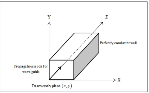
describes that only electric field propagates in the wave guides perpendicularly and called transverse electric (TEz).

3. Methodology

For solving full EM wave, 3-D analysis is required to determine the relation propagation mode dispersion. The geometry of closed type wave guide that z-axis direction and parameters of propagation β is shown as figure 1. The z-axis direction represents electric and magnetic field propagation. TM polarization to z-axis direction will be obtained

H

_z

(

x y z t

, , ,

)

=

0

, and TE polarization to z-axis direction will be obtained

E

_z

(

x y z t

, , ,

)

=

0

.

Cubical cell unit in the coordinate system is shown by figure 2. For each magnetic field component is surrounded by four components of electric field. And then for each electric field components is surrounded by four magnetic field. Time-stepping Finite Difference for electric and magnetic field can be obtained by analyzing six coupled scalar partialy differential equations. By using rectangle coordinate system,

E

_x

(

x y z t

, , ,

)

,

E

_y

(

x y z t

, , ,

)

, and

E

_z

(

x y z t

, , ,

)

that represents electric

components. Then for

H

_x

(

x y z t

, , ,

)

,

H

_y

(

x y z t

, , ,

)

, and

H

_z

(

x y z t

, , ,

)

that represents magnetic

Figure 1. Geometry of closed-type wave guide

x

D ,

D

y

, and Dz represents lattice special addition as long as x_{, y, and zcoordinate. The D}t represents additional time and

(

i j k

, ,

)

represents the location of

(

i x j y k z

D

,

D

,

D

)

.

Figure 2. Geometry of closed-type wave guide

The selecting of spatial additional _Dx_,

_D

_y

_{, and Dzalso time additional D}t_{are chosen because the} stability accurate and algorithm. For make sure the stability of computational field, _Dt_{is chosen to} fulfill inequality that expressed by these following equation:

1 2

2 2 2

max

1

1

1

1

t

c

x

y

z

-é

ù

D £

_ê

₊

₊

_ú

D

D

D

ë

û

(12)

where

c

maxis the maximum wave velocity.

4. Result and Discussion

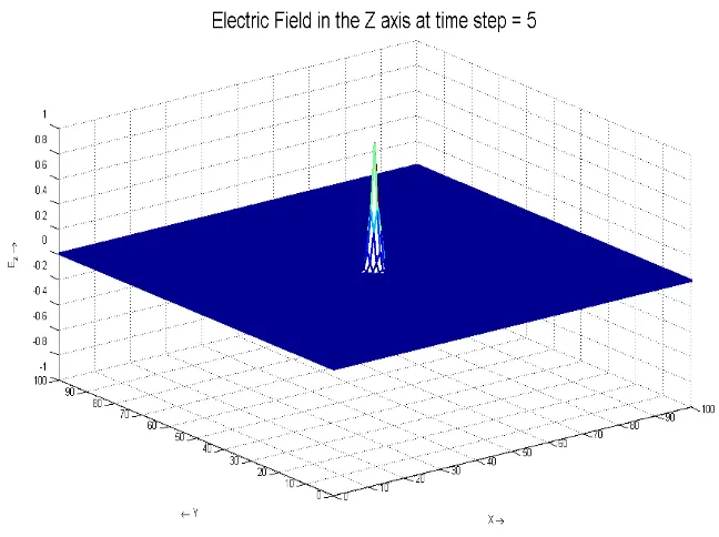
time-5

step of 150 computational times to observe the attenuation of electric field’s amplitude in the subsurface.

1. Sinusoidal Source

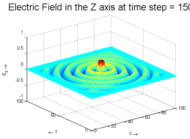
The electric current is generated from the transmitter as a sinusoidal function. The amplitude of electric current reaches the maximum value at the time-step is equal to zero. As the sinusoidal function, the electric current will decay and reaches the minimum value after reaches its maximum. This condition is shown by figure 3(a) and 3(b) that illustrate the changing of electric current intensity from maximum to minimum point. At time-step 150, the maximum and minimum amplitude is can be distinguished easily because the source of electric current is still generated by the transmitter as shown by figure 3(d).

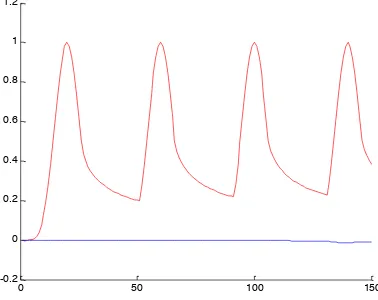
For a comparing between maximum and minimum value, we separate the maximum and minimum amplitude of electric field into two graphs, as shown by figure 3(c). Maximum and minimum value is can be analyzed the resistivity structure in that position. This model also can be applied to the real observed data from the geothermal field, so we can analyze the resistivity structure in the real condition of geothermal system.

Figu

Picture 3(b). The pattern of electric field for the sinusoidal source at time-step = 150

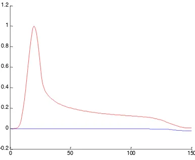
Figure 3(c). The maximum (red graph) and minimum (blue graph) amplitude of electric field at

time-step = 150

Figure 3(d). The maximum and minimum amplitude of source at time-step = 150

0 50 100 150

-1 -0.8 -0.6 -0.4 -0.2 0 0.2 0.4 0.6 0.8 1

0 50 100 150

7

2. Single Gaussian Source

This variation source is decaying faster than the first one. It’s happened because the source is generated only one time and almost be zero after reaches time-step 150, as shown figure 4(a). The maximum value will be attenuated to be almost zero or reaches the minimum point after reaches its maximum point as shown figure 4(b).

Figure 4(a). The pattern of electric field for the single gaussian source at time-step = 150

Figure 4(b). The maximum (red graph) and minimum (blue graph) amplitude of electric field at

time-step = 150

0 50 100 150

0 50 100 150 -0.2

0 0.2 0.4 0.6 0.8 1 1.2

Figure 4(c). The maximum and minimum amplitude of source at time-step = 150

3. Periodic Gaussian Source

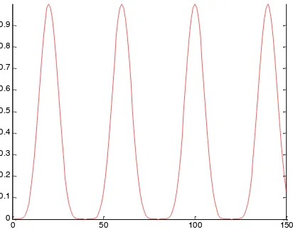
The amplitude of electric field is still observed at time step 150, compare to initial condition as shown by figure 5(a). This condition is occurred because electric current is generated by transmitter periodically, so we have only the maximum value that also generated periodically as shown by figure 5(b). If we compare figure 5(c) to picture 3(d), we can say that the maximum amplitude is generated periodically. But at the same time, which time-step is 150, sinusoidal source has propagated two times than periodic Gaussian source.

Figure 5(a). The pattern of electric field for the periodic gaussian source at time-step = 150

Figure 5(b). The maximum (red graph) and minimum (blue graph) amplitude of electric field at

time-step = 150

0 50 100 150

9

Figure 5(c). The maximum and minimum amplitude of source at time-step = 150

5. Conclusion

From this modeling that has been conducted, we can conclude that the amplitude of electric field will attenuate when it propagates in the earth. As shown by electric field propagating at time–step 150 we can see that the amplitude is decaying by the increasing of time. One of the reasonable for this attenuation is because there is an interaction between electric field and materials in the subsurface. This condition means that the resistivity structure in the subsurface is able to analyze by comparing the intensity or amplitude of electric and magnetic field. This information of electric field can be used for analyzing the resistivity structure by comparing to magnetic field that also propagates in the subsurface.

For the geothermal system, resistivity structure is very important to analyze the conductivity of rocks or geological structure in the layered earth. Conductivity gives us the information about the physical parameters such as the rock density, dimension of geothermal energy storage, and temperature of fluids or gases flow in the subsurface.

Propagation of EM field for TE mode is successfully conducted. We can analyze the source of geothermal prospect in the subsurface that can be explored for energy resources. This model also can be applied to the real observed data from the geothermal field, so we can analyze the resistivity structure in the real condition of geothermal system.

References

[1] Telford, W. M., Geldart, L. P., dan Sheriff, R. E. 1990. Applied Geophysics 2nd Edition. New York, Cambridge University Press

[2] Tikhonov, A. N. 1950. On Determining Electrical Characteristics of The Deep Layers of The Earth’s Chrust. Geophysical Institute Academy of Science, USSR, Reprinted from Doklady, 73, 2, 295-297

[3] Cagniard, L. 1953. Basic Theory of The Magnetotelluric Method of Geophysical Prospecting. Paris

[4] Zhdanov, M. S. 2010. Electromagnetic geophysics: Notes from the past and the road ahead. Geophysics, 75, 5 (2010); 75A49-75A66

[5] French, R. B. 2002. Time Domain Electromagnetic Exploration. Oregon: Northwest Geophysical Associated, Inc

[6] Ward, S. H. 1990. Geotechnical and Environmental Geophysics. Vol 2-Environmental and Groundwater. Society of Exploration Geophysicists. Tulsa-Oklahoma

[7] Fitterman, D. V. dan Stewart, M. 1986. Transient electromagnetic sounding for groundwater. Geophysics, 51 (April, 1986), 995-1005

[8] Papadopoulos, dkk. 2004. A TDEM survey to define local hydrogeological structure in Anthemountas Basin, N. Greece. Jurnal of Balkani Geophysical Society, 7, 1, Agustus 2004; 1-11

[10] Srigutomo, W. dkk. 2015. Time-domain electromagnetic (TDEM) baseline survey for CCS in Gundih area, Central Java, Indonesia. Proceedings of the 12th SEGJ International Symposium 2015

[11] Wang, T. dan Hohmann, G. W. 1993. A Finite-Difference, Time-Domain Solution for Three-Dimensional Electromagnetic Modeling. Journal of Geophysics, Vol. 58, No.6; P. 797-809 [12] Pridmore, D.F. dkk. 1981. An investigation of finite-element modeling for electrical and

electromagnetic data in three dimensions. Geophysics, 46, 7, July 1981; 1009-1024

[13] Sha, W. dkk. 2007. Application of The Simplectic Finite-Difference Time-Domain Scheme to Electromagnetic Simulation. Journal of Computational Physics 225 (2007) 33-50

[14] Rao, S. M. 1999. Time Domain Electromagnetics. A Harcourt Science and Technology Company, Academic Press