Full Terms & Conditions of access and use can be found at
http://www.tandfonline.com/action/journalInformation?journalCode=ubes20
Download by: [Universitas Maritim Raja Ali Haji] Date: 12 January 2016, At: 23:47
Journal of Business & Economic Statistics
ISSN: 0735-0015 (Print) 1537-2707 (Online) Journal homepage: http://www.tandfonline.com/loi/ubes20
Bias-Corrected Estimation in Dynamic Panel Data
Models
Maurice J.G Bun & Martin A Carree
To cite this article: Maurice J.G Bun & Martin A Carree (2005) Bias-Corrected Estimation in
Dynamic Panel Data Models, Journal of Business & Economic Statistics, 23:2, 200-210, DOI: 10.1198/073500104000000532
To link to this article: http://dx.doi.org/10.1198/073500104000000532
Published online: 01 Jan 2012.
Submit your article to this journal
Article views: 187
View related articles
Bias-Corrected Estimation in Dynamic
Panel Data Models
Maurice J. G. B
UNFaculty of Economics and Econometrics, University of Amsterdam, The Netherlands (m.j.g.bun@uva.nl)
Martin A. C
ARREEFaculty of Economics and Business Administration, University of Maastricht, The Netherlands (m.carree@os.unimaas.nl)
This study develops a new bias-corrected estimator for the fixed-effects dynamic panel data model and derives its limiting distribution for finite number of time periods,T, and large number of cross-section units,N. The bias-corrected estimator is derived as a bias correction of the least squares dummy variable (within) estimator. It does not share some of the drawbacks of recently developed instrumental variables and generalized method-of-moments estimators and is relatively easy to compute. Monte Carlo experi-ments provide evidence that the bias-corrected estimator performs well even in small samples. The pro-posed technique is applied in an empirical analysis of unemployment dynamics at the U.S. state level for the 1991–2000 period.
KEY WORDS: Bias correction; Dynamic panel data model; Unemployment dynamics.
1. INTRODUCTION
The estimation of fixed-effects dynamic panel data models has been one of the main challenges in econometrics during the last two decades. Various instrumental variables (IV) es-timators and generalized method-of-moments (GMM) estima-tors have been proposed and compared (see, e.g., Anderson and Hsiao 1981, 1982; Arellano and Bond 1991; Arellano and Bover 1995; Ahn and Schmidt 1995; Kiviet 1995; Wansbeek and Bekker 1996; Ziliak 1997; Blundell and Bond 1998; Hahn 1999; Judson and Owen 1999). The development and comparison of such new estimators was necessary because the traditional least squares dummy variable (LSDV) estimator is inconsistent for fixedT. Despite the increasing sophistication of the IV and GMM estimators, they have two important draw-backs. First, the complexity of the new estimators is a barrier for applied researchers (see, e.g., Baltagi, Griffin, and Xiong 2000). This should be only a temporary drawback, however, as the new estimators are incorporated into the statistical packages. But the newly developed estimators may require additional deci-sions on, for example, which and how many instruments to use. For example, by evaluating the expectation of asymptotic ex-pansions of estimation errors, Bun and Kiviet (2002b) showed that finite-sample bias of GMM estimators increases with the number of moment conditions used. This makes application less straightforward. In addition, the new estimators introduce problems of their own. For example, the performance of some GMM estimators depends strongly on the ratio of variance of the individual-specific effects and the variance of the general error term (see, e.g., Kitazawa 2001; Bun and Kiviet 2002b).
This article introduces a new and simple estimator for dy-namic panel data models with or without additional exogenous explanatory variables. An important advantage of this estima-tor is that it does not depend on the ratio of the variance of the individual-specific effects and the variance of the general error term. It is computed as a bias correction to the LSDV estimator (also referred to as the within estimator) and as such is related to estimators developed by Kiviet (1995), Hansen (2001), and Hahn and Kuersteiner (2002). MacKinnon and Smith (1998)
already indicated that bias of parameter estimates may be vir-tually eliminated in some common cases, albeit at the expense of increased variance of the estimators. The present article con-firms this for the case of dynamic panel data models. Regard-ing dynamic panel data models, Kiviet (1995) and Judson and Owen (1999) presented Monte Carlo evidence indicating that the bias-corrected estimator proposed by Kiviet (1995) may outperform IV and GMM estimators.
This article provides evidence of the usefulness of bias cor-rection, but the resulting estimator does not share some limita-tions of existing bias-corrected procedures. First, Kiviet (1995) proposed consistently estimating the extent of the bias by using a preliminary consistent estimator. This allows for a consistent corrected estimator based on additive bias correction. An obvi-ous disadvantage of such a procedure is that its finite-sample accuracy depends on the preliminary estimator chosen. Bias adjustment of the newly developed estimator is done without resorting to outside initial consistent estimates and appears to perform well in comparison. Second, Hansen (2001) proposed a somewhat similar bias-corrected estimator as in this study, but did not derive its limiting distribution. Also, the bias-correction procedure proposed by Hansen does not take into account the inconsistency of the LSDV estimator of the variance of the er-ror term. Finally, Hahn and Kuersteiner (2002) recently intro-duced a bias-corrected estimator related to that developed by Kiviet (1995); however, their estimator is not designed for sam-ples with smallT.
The rest of the article is organized as follows. In Section 2 we explain the principle of bias correction in dynamic panel data models. In Section 3 we derive the limiting distribution of the bias-corrected estimator for finiteT and largeN. In Section 4 we discuss the special case of the AR(1)model in which no additional exogenous variables are included. We compare the bias-corrected estimator with other possible corrections on the
© 2005 American Statistical Association Journal of Business & Economic Statistics April 2005, Vol. 23, No. 2 DOI 10.1198/073500104000000532
200
LSDV estimator. In Section 5 we present results from Monte Carlo experiments for the model with an additional exogenous regressor. In Section 6 we apply the estimators to a simple model of intertemporal dynamics of the unemployment rate in U.S. states in the 1991–2000 period. Finally, in Section 7 we discuss extensions and limitations of the proposed estimator in more general models and provide concluding remarks.
2. BIAS–CORRECTED ESTIMATION IN DYNAMIC PANEL DATA MODELS
In this section we illustrate the principle of bias-corrected es-timation in the first-order dynamic panel data model. For ease of exposition, we assume only one additional time-varying re-gressor (next to the lagged dependent variable rere-gressor) and the panel to be balanced. Consider the following first-order dy-namic panel data model
yit=γyi,t−1+βxit+ηi+εit, i=1, . . . ,N;t=1, . . . ,T. (1) In this model the dependent variable yit is determined by the one-period lagged value of the dependent variableyi,t−1, the
additional regressorxit, the unobserved individual-specific ef-fectηi, and a general disturbance termεit. The regressorxitmay be correlated with the individual-specific effectηi, but we as-sume that it is strictly exogenous with respect to the general er-ror termεit. Regarding the latter, we assume that it has mean 0, constant varianceσε2, and finite fourth moment, not correlated either over time or across individuals and not correlated withηi. Considering the startup observationsyi0, we assume that they
are uncorrelated with subsequent error termsεit. Finally, there are no assumptions about the value ofγ; that is, it is not neces-sary to assume that model (1) is dynamically stable.
The unknown individual effects in (1) can be eliminated by expressing each variable in deviation of its individual-specific mean. We introducey˜it=yit− ¯yi,y˜i,t−1=yi,t−1− ¯yi,−1, ˜
xit=xit− ¯xi, andε˜it=εit− ¯εiand rewrite model (1) as
˜
yit=γy˜i,t−1+βx˜it+ ˜εit, i=1, . . . ,N;t=1, . . . ,T. (2) We compute the LSDV estimators by applying ordinary least squares (OLS) to this equation to give
ˆ
The LSDV estimators ofγandβ are biased and inconsistent for fixedT because of the correlation betweeny˜i,t−1 and ε˜it. The extent of the inconsistency can be computed as follows. We rewrite (3) and (4) as From (1), we use continuous substitution to obtain
yit=γtyi0+β(xit+γxi,t−1+ · · · +γt−1xi1)
Note that this also holds for the specific case of γ =1, be-cause we have limγ→1(1−γt)/(1−γ )=t. To obtain an
ex-From this, it can be derived that whenyi0is uncorrelated with
subsequent error termsεit,
plim
This expression is always negative (for γ ≥ −1), because the function h(γ ,T)is positive. Having N tending to infinity and using plimN→∞N(T1−1) x˜itε˜it=0 (because the error
termε˜itis assumed to be uncorrelated withx˜it), we find that the inconsistency of the LSDV coefficient estimators equals (see also Nickell 1981, p. 1424; Kiviet 1995, p. 61)
γ∗= plim
We introduce the following expressions of the (asymptotic) variances of y˜i,t−1 and x˜it and their (limiting) covariance:
consistency of the LSDV coefficient estimators is now conve-niently expressed as
whereρxy−1=σxy−1/σxσy−1andζ =σxy−1/σ
From the first expression in (12), it is clear that the LSDV es-timator γˆlsdv is downward-biased. The extent of the
(as-ymptotic) bias depends on five parameters: γ, T, σε2, σy2
−1, andρxy2
−1. The bias of the LSDV estimator will be especially severe when (a) the value ofγ is close to 1 or even exceeds 1; (b) the number of time periods,T, is low; (c) the ratio of vari-ances,σε2/σy2
−1, is high; or (d) the lagged endogenous variable and the exogenous variable are highly correlated, either posi-tively or negaposi-tively. The second expression in (12) shows that the inconsistency of βˆlsdv is proportional to that ofγˆlsdv. The
bias of the LSDV estimatorβˆlsdvcan be either positive or
neg-ative, depending on the sign of the (asymptotic) covariance be-tweeny˜i,t−1andx˜it.
The principle of bias correction can be explained straightfor-wardly using (12). First, assume that we would know the values forσε2,ρxy−1,σ
2
y−1, andζ. Then we may use as a bias-corrected estimator,γˆbc(where the subscriptbcmeans “bias-corrected”;
the fact thatbcalso are the initials of the authors’ surnames is purely coincidental), that value ofγ for which
ˆ
This estimator can then be inserted into the second expres-sion in (12) to find the bias-corrected estimator βˆbc= ˆβlsdv+
ζ (γˆlsdv− ˆγbc). The functionh(γ ,T)as defined in (9) plays an
important role in this nonlinear bias-correction procedure. This function is always positive and monotonically increasing for γ≥ −1, a condition that usually can be safely assumed to hold in applications. Forγ=1, the functionh(γ ,T)has a value of
h(1,T)=1/2 (using l’Hôpital’s rule) irrespective of the length of time periodT. ForT=2, the functionh(γ ,2)is equal to 1/2, and forT=3, the functionh(γ ,3)is equal to(2+γ )/6. Hence forT=2, the bias-corrected estimator can be expressed explic-itly as
ForT=3, it can be expressed explicitly as
ˆ
For T >3, (13) must be solved numerically. Equation (13) can for example be solved numerically as follows. Define
C=σε2/(1−ρxy2
−1)σ
2
y−1 and takeγˆ(0)= ˆγlsdv. An iterative pro-cedure to converge toward the bias-corrected estimate (from be-low) isγˆ(j+1)= ˆγlsdv+Ch(γˆ(j),T).
In practice, we do not know the values forσε2,ρxy−1,σ
2
y−1, andζ. The values of the latter three variables can be estimated consistently using their sample analogsρˆxy−1 = ˆσxy−1/σˆxσˆy−1,
inconsistent, and the variance of the error term can be consis-tently estimated only when the LSDV estimators for γ andβ have been bias-corrected. We discuss three solutions to this
problem that lead to the same bias-corrected estimates. First, we can use an iterative procedure for (13). We then substitute the LSDV estimate forσε2in (13) to achieve one-step estimates for γ and β. These estimates are used to compute the one-step estimate forσε2. This one-step estimate is again substituted in (13) to achieve two-step estimates forγ andβ and so on un-til convergence. Second, an alternative procedure is to use the expression for the inconsistency of the LSDV estimate forσε2, that is,
is then substituted into (13) to arrive at an expression from whichγˆbccan be derived in one step, that is,
Equation (17) can, for example, be solved numerically as fol-lows. DefineC= ˆσlsdv2 /(1−ρxy2
−1)σ
2
y−1 and take γˆ(0)= ˆγlsdv. An iterative procedure to converge toward the bias-corrected estimate isγˆ(j+1)= ˆγlsdv+2h(γˆ1
(j),T)(1−
√
1−4Ch(γˆ(j),T)2).
ForT =2, an analytic expression for the bias-corrected esti-mate can be derived as
ˆ
Finally, to achieve bias-corrected estimates,σε2in equation (13) can be replaced by the infeasible estimate (we are grateful to a referee for suggesting this procedure)
˜
σε2= (y˜it−γy˜i,t−1−β˜xit)
2
N(T−1) , (19)
and we solve the following equivalent of (12) forγ andβ si-multaneously:
At first sight, this procedure would appear more cumbersome because there is an optimization with two arguments (γandβ) instead of one argument (γ). However, there is an advantage to deriving the expression for (asymptotic) standard errors, be-cause the (asymptotic) distribution of σˆlsdv2 is not necessary. Using any one of the iterative procedures (13), (17), or (20) results in the same bias-corrected estimate,γˆbc,βˆbc, orσˆbc2.
3. ASYMPTOTIC PROPERTIES OF BIAS–CORRECTED ESTIMATORS
In this section we discuss the asymptotic properties of the proposed bias-corrected estimators. We derive consistency and asymptotic normality for the corrected estimators for fi-nite T and N large. We generalize the discussion to the case withK additional exogenous variables,x1it throughxKit, and use matrix notation. Stacking the observations over time, that is,yi=(yi1, . . . ,yiT)′,yi,−1=(yi0, . . . ,yi,T−1)′,β=(β1, . . . , mator for model (22) is equal to
ˆ is the within-transformation matrix that eliminates the individ-ual effects andˆxy,ˆxx,σˆy−1y, andˆxy−1 are sample analogs of xy =plimN→∞N(T1−1)X′Ay, xx=plimN→∞N(T1−1) × X′AX, σy−1y = plimN→∞N(T1−1)y′−1Ay, and xy−1 = plimN→∞N(T1−1)X′Ay−1.
Define the inconsistency of the LSDV estimator as δ∗ = plimN→∞(δˆlsdv −δ). We now introduce ρXy2 −1 =
′
xy−1 × −xx1xy−1/σ
2
y−1 as the (asymptotic) squared multiple correla-tion coefficient of the regression ofy˜i,t−1onx˜1it throughx˜Kit andζ=(ζ1, . . . ,ζK)=−xx1xy−1 as the corresponding vector of regression coefficients. This allows us to generalize (12) and express the inconsistencyδ∗=(γ∗,β∗′)′as Although inconsistent, the LSDV estimator has a limiting distribution forN → ∞and fixed T. Bun and Kiviet (2001) derived the limiting distribution as
√ with the first element equal to 1 and the other elements equal to 0, andz(γ ,T)equal to sion for the inconsistency holds irrespective of the distribution of the error term εit. However, the specific expression for the matrixVX holds under normality of the error term only. Using
notation introduced earlier, the variance–covariance matrixVX
of the limiting distribution (25) of the LSDV estimator can be expressed as
The result (25) of Bun and Kiviet (2001) showed that the LSDV estimator has a limiting normal distribution for finite T
andN→ ∞, but it is not centered atδ, and it has a nonstandard variance–covariance matrix.
We now turn to bias-corrected estimation of δ=(γ ,β′)′. We first assumeσε2to be given. Generalizing the results of Sec-tion 2 [see (13)], using (24), the bias-corrected estimator forγ is thatγ which solves
ˆ
The resulting estimator can then be inserted into the second ex-pression in (24) to find the bias-corrected estimator for β. In short, we solveδˆlsdv=g(δ)forδwith
where σy2
−1|X =(1−ρ
2
Xy−1)σ
2
y−1 is the conditional variance of y˜−1. Defining f(δ)=g−1(δ), the expression for the
bias-corrected estimator is
ˆ
δbc=f(δˆlsdv). (32)
The functionfis unknown but can be evaluated numerically us-ing only a few lines of computer code; for details, see Section 2.
From (32), we see that
plim
and hence the bias-corrected estimator is a consistent estimator ofδfor finiteT andN→ ∞. Furthermore, exploiting (25) and using the delta method, we have
√ atives of the vector function f. Hence the bias-corrected esti-mator (32) has a limiting normal distribution centered atδ. Its asymptotic variance depends onVXandF. The latter matrix is
simplyF=G−1with
Using results on partitioned matrix inversion, the matrix
F=G−1can be written as
This implies that the first diagonal element of the matrixFVXF′,
orN∗var(γˆbc), is simply equal toVX11/(1−σε2h′(γ )/σy2−1|X)
2
and thatN∗var(βˆbc)is equal toVX22. ForT=2, the matrixF
equals the unity matrixI, because thenh′(γ )=0.
In general, σε2 is unknown and also must be estimated. There are at least three equivalent approaches leading to the same bias-corrected estimator; see Section 2 for details. First, we can use an iterative procedure. Second, we can extend δ toδ=(γ ,β′, σε2)′. Exploiting (16), we now solveδˆlsdv=g(δ) We then have that (31) is replaced by
g(δ)=
The corresponding matrixGis then derived as
G= evaluated for the bias-corrected estimators, somewhat simpli-fying calculation ofG. We use this last approach to compute asymptotic standard errors in the simulation and empirical ex-ercises. They are estimated consistently by N1FˆVˆXFˆ′using the
bias-corrected estimators andFˆ= ˆG−1. We now turn to the spe-cific case of having no additional exogenous variables.
4. BIAS–CORRECTION IN THE PANEL AR(1) MODEL
In this section we apply the limiting distribution theory of the previous section to a special case, the first-order dynamic panel data model without additional exogenous variables. We analyze the model
yit=γyi,t−1+ηi+εit, i=1, . . . ,N;t=1, . . . ,T. (38)
This model is a special case of (21) whereβ=0. An important difference from the preceding sections is that here we make ex-plicit assumptions about the admissible values forγ and about the distribution of the initial observations yi0. Regarding γ,
we now assume that|γ|<1, and for the initial observations, we assume that the process (38) has been going on for a long time, that is,
with the same assumptions aboutεi0as for the other disturbance
termsεit,t=1, . . . ,T (see Sec. 2). Note that this specific as-sumption about yi0 matches our earlier assumption about the
initial observations made in Section 2; that is, allNstartup ob-servationsyi0are uncorrelated with allεit fort>0. However, the additional assumptions aboutγ andyi0enable us to derive
explicit expressions for the inconsistency of the LSDV estima-tor and its asymptotic variance as a function of γ and T, as we discuss later. This makes it possible to analytically com-pute and compare the asymptotic efficiency of original and bias-corrected LSDV estimators.
Stacking the observations over time and across individuals, we get
y=γy−1+(IN⊗ιT)η+ε. (40)
Focusing on the autoregressive parameter γ, estimation of model (40) by OLS yields
ˆ
γlsdv=(y′−1Ay−1)−1y′−1Ay=γ+(y′−1Ay−1)−1y′−1Aε. (41)
The inconsistency of the LSDV estimator forγ whenN tends to infinity can be expressed as (Nickell 1981; Hsiao 1986)
γ∗= plim
Note that the inconsistency of the LSDV estimator is a func-tion ofγfor fixedTand does not depend onσε2; that is, we have plimN→∞(γˆlsdv)=γ∗+γ =g(γ ) for given T. In the
inter-val[−1,1), the functiongis a monotonically increasing func-tion of γ with minimum value g(−1)= −1 and maximum value g(1)=1−3/(T+1), the latter of which is computed using l’Hôpital’s rule. Hence it is possible to invert the func-tiongand expressγ as a function of plimN→∞(γˆlsdv), that is,
γ =f(plimN→∞(γˆlsdv))withf =g−1. Analogous to previous
sections, a consistent bias-corrected estimator thus can be con-structed as
ˆ
γbc=f(γˆlsdv). (43)
For example, when T = 2, we find from (42) that plimN→∞(γˆlsdv)=(γ −1)/2. Hence we use 2γˆlsdv+1 as a
bias-corrected estimator forγ. However, for higher values ofT, the functionf is unknown but can be evaluated numerically or approximated by a known function. However, in the latter case consistency is lost, due to the approximation. Carree (2002) proposed approximating the function f by a linear specifica-tion. His estimate is easy to calculate but requires using a table to obtain values for the intercept and slope. Furthermore, the estimator is inconsistent forN→ ∞, due to the approximation. These properties make this estimator less appealing.
We now turn to limiting distributions of the LSDV estimator and the proposed bias-corrected estimator. Exploiting (25), the limiting distribution forγˆlsdvfor finiteT and largeNis
√
ε. Using equation (14) of Nickell
(1981), we have that Regarding the bias-corrected estimator (43), we find, us-ing (33), that
The asymptotic variance depends on V and the first deriv-ative of the function g. Evaluating the latter factor analyti-cally is cumbersome, but it can be approximated numerianalyti-cally. In fact, to compute the variance of γˆbc, we insert this
esti-mate into (45) to find Vˆ. We then approximate the first deriv-ative of g using the expression forγ∗(γ )as given in (42) by
g′(γˆbc)=1+ [γ∗(γˆbc)−γ∗(γˆbc−µ)]/µ, withµa small
num-ber, say .001. We could also actually derive the analytic first derivative from (42), but this is not an elegant expression.
For the dynamic panel data model without additional ex-ogenous regressors (38), other estimators can be used that are not consistent for fixed T but are simple to compute, being linear functions of the LSDV estimator. It is interest-ing to compare their asymptotic efficiency with that of the
ˆ
γbc estimator. A first estimator emerges from taking a
lin-ear approximation to (42). When we insert in (42) values for γ equal to 0 and 1 (using l’Hôpital’s rule), we find that for γ =0, plimN→∞(γˆlsdv)= −1/T and that for γ → 1,
The estimator in (47) strongly resembles an estimator proposed by Hahn and Kuersteiner (2002),
ˆ
Although the estimators (47) and (48) are also inconsistent for finite T, the leading bias term of order O(T−1)has been ac-counted for. Hence these estimators may perform reasonably well for moderateT.
Each of the three estimators (43), (47), and (48) are functions ofγˆlsdv, for which we know the limiting distribution (44), which
is dependent onγ andT. This makes it possible to analytically compute asymptotic bias and variance of the estimators. These are presented in Table 1 for values ofTequal to 3, 6, and 10 and values ofγ equal to 0, .4, and .8. The bias-corrected estimator
ˆ
γbchas (by definition) the lowest bias, whereas the Hahn and
Kuersteiner estimator has considerable bias for small T. The latter estimator has the lowest asymptotic variance of the three estimators, however. In terms of mean squared error (MSE),
ˆ
γbcwould be preferable if we had smallTandNlarge, because
the extent of bias would dominate this measure for such dimen-sions.
5. MONTE CARLO EXPERIMENTS
In this section we compare the performance of the bias-corrected estimator (32), denoted by bc, with some alterna-tive estimators in a first-order dynamic panel model with an additional exogenous regressor. We comparebcwith the orig-inal LSDV estimator (lsdv), an additive bias-corrected esti-mator (ac), and the GMM estimator (gmm) of Arellano and Bond (1991). For ac, we use a slightly different version of Kiviet’s (1995) estimator in which there is bias correction of the first-order term only. Bun and Kiviet (2002a) showed
Table 1. Asymptotic Bias and Variance for the Panel AR(1) Model
T γ γ∗ g′ V N*var(γˆbc) bias(γˆc) N*var(γˆc) bias(γˆhk) N*var(γˆhk)
3 0 −.333 .611 .444 1.191 0 1.306 −.111 .790
3 .4 −.494 .587 .607 1.763 .010 1.785 −.192 1.080
3 .8 −.663 .569 .814 2.513 .006 2.391 −.284 1.447
6 0 −.167 .811 .174 .265 0 .320 −.028 .237
6 .4 −.251 .762 .161 .278 .028 .296 −.059 .219
6 .8 −.361 .684 .146 .312 .020 .268 −.121 .198
10 0 −.100 .891 .101 .128 0 .148 −.010 .123
10 .4 −.148 .864 .086 .116 .026 .126 −.023 .104
10 .8 −.218 .768 .051 .087 .024 .075 −.060 .062
NOTE: The asymptotic bias(γˆbc) is always equal to 0. The value forVisN∗var(γˆlsdv).
that this first-order term is responsible for most of the finite-sample bias in the LSDV estimator. We use the GMM es-timator as the first-step–consistent estimate. Assuming strict exogeneity of xit, we have T(T −1)/2+T(T −1) moment conditions for gmm, that is, E[yi,t−sεit] =0 (t=2, . . . ,T;
s=2, . . . ,t) and E[xisεit] =0 (t=2, . . . ,T;s=1, . . . ,T). We do not exploit additional moment conditions due to im-posing homoscedasticity, because Ahn and Schmidt (1995) noted that efficiency gains are small. Regarding the strict ex-ogeneity of xit to economize on the number of moment con-ditions, we also experimented with a GMM estimator using
E[yi,t−sεit] =0 (t=2, . . . ,T;s=2, . . . ,t) andE[x′iεi] =0, and hence T(T−1)/2+1 moment conditions. However, this resulted in lower efficiency, that is, higher root mean squared error (RMSE). Under the assumptions made in Section 2, the GMM estimator is consistent for finiteTand largeN, and hence it is a reasonable benchmark for evaluating the corrected LSDV variants.
We generated data foryaccording to (1) withηi∼IIN[0, ση2]andεit∼IIN[0, σ2
ε]. The generating equation for the
ex-planatory variablexis
xit=ρxi,t−1+ξit, i=1, . . . ,N;t=1, . . . ,T, (49)
where ξit ∼IIN[0, σ2
ξ]. We used three different research
designs. In the first design we chose β =1, ρ =.8, and ση=σε=σξ=1. We used two different values forγ, .4 and .8.
We assumed that the panel dataset comprises 600 observations and conducted experiments for several combinations ofTandN
for whichNT=600. The second design was equal to the first design, except that we allowed for time series heteroscedastic-ity in the general error term εit. (We also experimented with cross-sectional heteroscedasticity in the general error termεit, but the results were qualitatively not very different from those obtained in the first design.) In this design,σε2is varying over time; that is, we specifyσε2,t=.95−.05T+.1t. This specifica-tion ensures that T1T
t=1σε2,t=1; hence a proper comparison can be made with the simulation results in case of homoscedas-ticity. The third research design has identical parameter settings to the design used by Kiviet (1995, table 1). In all of Kiviet’s ex-periments the long-run effectβ/(1−γ )ofxonyis set equal to unity, and hence the impact multiplierβvaries with the chosen values forγ. Homoscedasticity is assumed, and the value ofσε2 is set equal to 1, but the values of the variancesση2andσξ2differ across experiments. By varyingση2, the relative impact onyof the two error componentsηandεis changed, whereas the para-meterσξ2determines the signal-to-noise ratio of the model (for
details, see Kiviet 1995). For each experiment, we performed 10,000 Monte Carlo replications.
Selected simulation results for the first, second, and third de-signs are presented in Tables 2–4. Regarding coefficient esti-mators, these tables present in the bias in estimatingγ andβ together with the RMSE. In calculating the RMSE of coefficient estimators, we use the variance as estimated from the Monte Carlo as a measure of true variance. Next to bias and RMSE, we report actual size of (two-sided) simplet-tests of the para-metersγ orβ to be equal to the values chosen in the respec-tive designs. The nominal size is 5% for each research design. Actual size is calculated as the percentage of replications for which the ratio of coefficient estimator and its standard devi-ation estimator is larger than 1.96 in absolute value. Regard-ing the variance estimators used to calculate tratios, forlsdv
andacwe use the standard variance expression,σˆε2(W′AW)−1. Forbc, we use the expression in (33) (unreported simulation
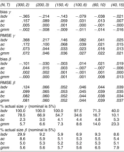
Table 2. Homoscedasticity,γ=ρ=.8 andβ=1
(N, T) (300, 2) (200, 3) (150, 4) (100, 6) (60, 10) (40, 15)
biasγ
lsdv −.365 −.214 −.143 −.079 −.038 −.021 ac .157 .089 .059 .031 .013 .007 bc .005 .000 .001 .000 −.001 −.000 gmm −.002 −.008 −.009 −.011 −.014 −.016 RMSEγ
lsdv .368 .217 .146 .082 .041 .025 ac .172 .100 .068 .039 .021 .015 bc .073 .044 .033 .023 .016 .013 gmm .072 .046 .036 .027 .022 .021 biasβ
lsdv −.101 −.030 −.003 .014 .021 .019 ac .044 .015 .003 −.007 −.007 −.006 bc .002 .002 .001 −.001 .001 .000 gmm −.000 .000 .001 .001 .008 .013 RMSEβ
lsdv .124 .066 .052 .046 .044 .039 ac .099 .065 .053 .045 .039 .035 bc .082 .060 .052 .044 .038 .034 gmm .081 .060 .052 .044 .039 .037 % actual sizeγ(nominal is 5%)
lsdv 100.0 100.0 100.0 97.5 71.3 40.0
ac 78.5 66.9 54.7 34.6 16.7 10.1 bc 2.3 3.0 4.1 4.4 4.8 5.3 gmm 5.7 6.6 7.3 8.6 14.0 23.3 % actual sizeβ(nominal is 5%)
lsdv 29.9 9.2 5.9 6.9 9.3 8.6 ac 8.6 5.9 5.1 5.3 5.5 5.4 bc 5.0 5.3 5.2 5.2 5.3 5.1 gmm 5.6 5.6 5.7 5.6 6.5 7.9
NOTE: For the variances, we assume thatσ2
ε=ση2=σξ2=1.
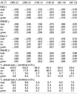
Table 3. Time Series Heteroscedasticity,γ=ρ=.8 andβ=1
(N, T) (300, 2) (200, 3) (150, 4) (100, 6) (60, 10) (40, 15)
biasγ
lsdv −.353 −.203 −.133 −.072 −.033 −.018 ac .178 .104 .071 .040 .019 .011 bc .035 .020 .015 .010 .005 .003 gmm −.002 −.008 −.009 −.010 −.013 −.014 RMSEγ
lsdv .356 .206 .136 .075 .036 .022 ac .192 .114 .079 .046 .025 .017 bc .084 .050 .037 .025 .017 .013 gmm .072 .046 .036 .026 .021 .020 biasβ
lsdv −.098 −.029 −.003 .013 .018 .015 ac .050 .017 .003 −.008 −.010 −.009 bc .010 .005 .001 −.003 −.002 −.003 gmm −.000 .001 .001 .001 .007 .012 RMSEβ
lsdv .121 .066 .052 .046 .042 .038 ac .102 .066 .054 .045 .039 .036 bc .084 .061 .052 .044 .038 .034 gmm .081 .060 .052 .044 .039 .037 % actual sizeγ(nominal is 5%)
lsdv 100.0 100.0 99.9 94.2 59.5 29.2
ac 86.1 77.9 68.0 48.5 25.4 15.4 bc 1.1 3.0 4.7 5.8 5.7 6.0 gmm 5.8 6.4 7.0 8.1 12.8 21.1 % actual sizeβ(nominal is 5%)
lsdv 28.0 8.8 5.9 6.7 8.5 7.5 ac 9.4 6.0 5.1 5.5 6.0 5.9 bc 4.9 5.3 5.2 5.1 5.3 5.0 gmm 5.6 5.6 5.7 5.5 6.7 7.7
NOTE: We assume thatσ2
ε,t=.95−.05T+.1tandση2=σξ2=1.
results show that the accuracy oft-tests based on thebc esti-mator depends on the normality assumption needed to derive asymptotic standard errors), whereas forgmm, we exploit the so-called one-step estimates.
Regarding the first design, Table 2 presents the results for γ=.8. The results forγ=.4 are similar and hence are deleted to save space. We observe the following patterns in the simula-tion results for the coefficient estimators. First, bias in estimat-ing the autoregressive parameterγ is always negative forlsdv
andgmm, whereas positive bias has been found forac. Second, for (bias-corrected) LSDV, the bias in estimating bothγ andβ decreases for larger T (and smallerN), but not so for gmm. This is to be expected becausegmm should perform well, es-pecially forT small andN large. Third, especially forγ, bias ingmmcarries over to bias inac, demonstrating the dependence of additive bias correction on preliminary consistent estimators. Fourth, in estimating bothγ andβ,bc is virtually unbiased. Finally, based on a MSE criterion,bcis almost never beaten by the other coefficient estimators. Regarding simplet-tests forbc, we observe that the actual size is close to the nominal size in most cases (except forγ in the case of smallT, when the actual size is somewhat low), indicating the accuracy of the asymp-totic approximation in this design.
Table 3 presents simulation results for the second design with time series heteroscedasticity. Again, we show the results for γ =.8 only. In general, results for bias-corrected estimators (acandbc) are worse here than in the case of homoscedasticity. This is not surprising, because bias-corrected estimators are not consistent in cases of time series heteroscedasticity. The addi-tive bias-corrected estimatoracis especially vulnerable to the
presence of heteroscedasticity, but the detrimental effects onbc
seem modest. Based on an MSE criterion, bc is now some-times beaten bygmm, especially for smallerT. The actual size forbcis still quite close to the nominal size of 5% (except for testingγ whenT=2).
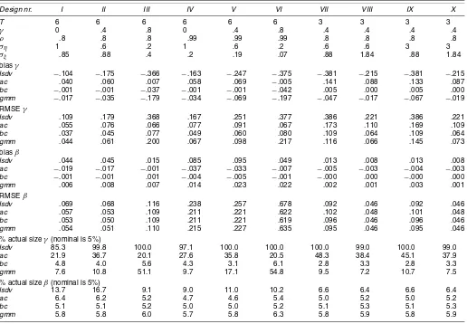
Finally, we turn to simulation results using the third design, that is, the parameterizations used by Kiviet (1995). Table 4 presents the simulation results for a selection of parameteri-zations. The first part of the table gives the parameterizations used. We need to make several points before discussing the sim-ulation results. First, the relative impact onyitof the two error componentsηiandεitis 1 in experiments I–VIII, but increases to 5 in experiments IX and X. Hence the individual-specific ef-fect is relatively strong in experiments IX and X. Second, the signal-to-noise ratio corresponds to an expected R2 of 2/3 in all experiments except VIII and X, where it increases to 8/9.
Regarding the third design, we observe the following pat-terns for the coefficient estimators. First, except for ac, bias in estimating the autoregressive parameterγ increases withγ for all estimators. Especially for larger values of γ, substan-tial coefficient bias is found for gmm. Second, there is no one estimation method with the lowest RMSE across all parameteri-zations. The bias-corrected estimator performs well in all of the designs except designs III and VI, in which there is a relatively high value forγ combined with a relatively low signal-to-noise ratio. The bias-corrected estimator fails to converge in about 40% of the replications in these two designs. We decided to skip such replications completely for each of the estimators. In all other experiments, we found very limited or no convergence problems. We also simulated designs III and VI withN=1,000 and found much less convergence problems (around 5%), indi-cating that this is a small sample issue. Regarding simplet-tests in the third design, we observe that forbc, again actual size is quite close to nominal size, whereas coefficient bias of other estimators clearly carries over to the accuracy oft-tests.
Summarizing, regarding coefficient estimators and sim-ple t-tests, we find large bias for lsdv, moderate bias for
ac and gmm, and little bias for bc. In addition, based on an RMSE criterion, the bias-corrected estimator performs comparatively well for a range of parameter combinations. However, the Monte Carlo results do not suggest that one es-timation technique is superior for all parameter combinations. Hence in empirical applications, it may be advisable to compare results using different (consistent) estimation techniques.
6. EMPIRICAL APPLICATION: UNEMPLOYMENT DYNAMICS AT THE U.S. STATE LEVEL
In this section we apply the bias-corrected estimation pro-cedure (denoted by bc) to a model of unemployment dynam-ics at the U.S. state level. We compare the coefficient estimates and estimated standard errors with those of the LSDV, additive bias-corrected LSDV, and GMM estimators (denoted by lsdv,
ac, and gmm); see the previous section for more details. As a benchmark, we included also the pooled OLS estimator (ols) in the empirical analysis.
The model relates the current unemployment rate (Uit) to the unemployment rate and economic growth rate (Git) in the pre-vious year. The model includes individual-specific and time ef-fects (ηiandλt),
Uit=γUi,t−1+βGi,t−1+ηi+λt+εit. (50)
Table 4. Simulation Results for Selected Designs From Kiviet (1995)
Design nr. I II III IV V VI VII VIII IX X
T 6 6 6 6 6 6 3 3 3 3
γ 0 .4 .8 0 .4 .8 .4 .4 .4 .4
ρ .8 .8 .8 .99 .99 .99 .8 .8 .8 .8
ση 1 .6 .2 1 .6 .2 .6 .6 3 3
σξ .85 .88 .4 .2 .19 .07 .88 1.84 .88 1.84
biasγ
lsdv −.104 −.175 −.366 −.163 −.247 −.375 −.381 −.215 −.381 −.215 ac .040 .060 .007 .058 .069 −.005 .141 .088 .133 .087 bc −.001 −.001 −.037 −.001 −.001 −.042 .005 .000 .005 .000 gmm −.017 −.035 −.179 −.034 −.069 −.197 −.047 −.017 −.067 −.019 RMSEγ
lsdv .109 .179 .368 .167 .251 .377 .386 .221 .386 .221 ac .055 .076 .066 .077 .091 .067 .173 .110 .169 .109 bc .037 .045 .077 .049 .060 .080 .109 .064 .109 .064 gmm .044 .061 .200 .067 .098 .217 .116 .066 .145 .073 biasβ
lsdv .044 .045 .015 .085 .095 .049 .013 .008 .013 .008 ac −.019 −.017 −.001 −.037 −.033 −.007 −.005 −.003 −.004 −.003 bc −.001 −.001 .001 −.004 −.005 −.001 −.000 .000 −.000 .000 gmm .006 .008 .007 .014 .023 .022 .002 .001 .003 .001 RMSEβ
lsdv .069 .068 .116 .238 .257 .678 .092 .046 .092 .046 ac .057 .053 .109 .211 .221 .622 .102 .048 .101 .048 bc .053 .050 .109 .211 .221 .619 .096 .046 .096 .046 gmm .054 .051 .110 .215 .227 .635 .095 .046 .095 .046 % actual sizeγ(nominal is 5%)
lsdv 85.3 99.8 100.0 97.1 100.0 100.0 100.0 99.0 100.0 99.0
ac 21.9 36.7 20.1 27.6 35.8 20.5 48.3 38.4 45.1 37.9
bc 4.8 4.0 5.6 4.3 3.1 6.1 2.8 3.3 2.8 3.3
gmm 7.6 10.8 51.1 9.7 17.1 54.8 9.5 7.2 10.7 7.5 % actual sizeβ(nominal is 5%)
lsdv 13.7 16.7 9.1 9.0 11.0 10.2 6.6 6.4 6.6 6.4
ac 6.4 6.2 5.2 4.7 4.6 5.4 5.0 5.2 5.0 5.2
bc 5.1 5.1 5.2 5.0 5.0 5.2 5.1 5.3 5.1 5.3
gmm 5.8 5.8 6.0 5.7 5.8 6.3 5.8 5.9 5.8 5.9
NOTE: We assume thatσ2
ε=1,N=100, andβ=1−γin all experiments.
Equation (50) can be rewritten in an easier-to-interpret, from, Uit=(γ−1)(Ui,t−1−αi)+β(Gi,t−1−δ)+λt+εit, (51) where (1−γ )αi−βδ=ηi. Equation (51) indicates that the change in the unemployment rate is determined by an adjust-ment of the unemployadjust-ment rate toward a “natural” or “equilib-rium” rate of unemployment, αi, which may differ across the states, and by the previous economic growth rate. The speed of adjustment of the unemployment rate toward the “natural” or “equilibrium” rate is equal to 1−γ. Partial adjustment, 0< γ <1, is expected. A state that has relatively high eco-nomic growth is more likely to have reduced unemployment rates compared with states in which the economy is growing more slowly. This would imply thatβ <0.
The data for the unemployment rate for the 1991–2000 pe-riod are obtained from the U.S. Bureau of Labor Statistics, and data for the (current dollar) gross state product are obtained from the U.S. Bureau of Economic Analysis. The economic growth rate is taken to be the relative growth of the gross state product. Data are available for all U.S. states and Washing-ton, DC (N=51). The number of time periods in estimation isT=9, because the year 1991 is taken as the starting observa-tion.
Table 5 presents the various coefficient estimates and their estimated standard deviations. The value of the LSDV esti-mate of γ is .484, which would imply an adjustment rate
of around 50% per year. In contrast, the bias-corrected esti-mate (bc) is equal to .615, which implies an adjustment rate of less than 40%. Hence the speed of adjustment toward a “natural rate of unemployment” is not as large as the original LSDV es-timator would suggest. The value of the LSDV estimate ofβ equals−.064, whereas the value of the bias-corrected estimate is−.057. This implies a somewhat smaller effect of economic growth on the change in unemployment than indicated by the traditional within estimate. The results for the additive bias-corrected estimator (ac) are somewhat different from those of the bias-corrected estimator introduced in this article. However, the results for the GMM estimator (gmm) are more or less equal to that ofbc.
A restrictive assumption of bias-corrected LSDV estimators is that consistency depends on strict exogeneity of the lagged growth rate,Gi,t−1. Because we have assumed strict exogeneity
Table 5. Empirical Results for the Unemployment-Growth Model
ols lsdv ac bc gmm
ˆ
γ .840 .484 .763 .615 .600
sd(γˆ) .022 .037 .040 .047 .048
ˆ
β −.041 −.064 −.049 −.057 −.057
sd(βˆ) .008 .012 .013 .012 .013
NOTE: T=9 andN=51; time dummies are included.
of Gi,t−1in GMM estimation, we can test against exogeneity
using the Sargan test. To increase power, we do not use all mo-ment conditions, onlyE[Ui,t−sεit] =0 (t=2, . . . ,T;s=2,3) and E[Gi,t−1εit] =0 (t=2, . . . ,T). The test has a value
of 25.09 (p value .29), and hence the validity of the mo-ment conditions is not rejected. We conclude that the problem ofGi,t−1 being only weakly exogenous is not an issue in this
particular application.
7. EXTENSIONS AND CONCLUDING REMARKS
In this article we have developed a new bias-corrected esti-mator for dynamic panel data models. The proposed estiesti-mator has desirable asymptotic properties for finiteTand largeN, but these have been derived under certain restrictive assumptions, including strict exogeneity of regressors inxit, homoscedastic-ity of the disturbances, and balanced panels. In this final sec-tion we discuss the limitasec-tions and possible extensions of our approach with respect to each of these three assumptions.
First, regarding the exogeneity assumption, some regressors inxit could be predetermined as well. Inconsistencies originat-ing from this source are not accounted for in the current bias corrections. It can be shown that the order of magnitude of such inconsistency terms equals that of lagged dependent variable regressors, that is, of orderO(T−1). But addressing the impor-tance of this source of bias requires full specification of the marginal process of the regressorsxit,which is a major com-plication in practice. Simulation evidence for the dynamic panel data model with predetermined or endogenous regressorsxithas been given by Bun and Kiviet (2002b) and Blundell, Bond, and Windmeijer (2000). In general, these simulation results show that lack of strict exogeneity of xit does influence the finite-sample properties of estimators, and hence it is expected that in practice estimators will be affected as well. Note, however, that in the current application on unemployment dynamics, strict exogeneity of the additional regressor (lagged growth rate) is not rejected. Second, regarding homoscedasticity of the distur-bances, we have provided some simulation results allowing for either cross-section or time series heteroscedasticity. From the simulation results, we see that in the latter case, bias-corrected estimators behave somewhat worse, as expected.
Finally, the proposed method in this study can be extended to unbalanced panels. In this case not all time observations are available for each individual i. That is, the data may be ob-served for certain individualsionly from a certain date, or the data may be observed for other individuals only up until a cer-tain date. This implies that the starting date and ending date of the data are individual-specific. Denoting the beginning of the data period byBiand the final time period of observation byTi, we have 1≤Bi≤Ti≤T. We then order the individuals in terms of the length of the time period,Ti−Bi+1. The largest value for this length of time period isT, and the smallest value is 2. Denote byϕt the fraction of observations with period of time lengtht=2, . . . ,T; that is,T
t=2ϕt=1. Then we replace the functionh(γ )in Sections 2 and 3 with
hu(γ )= T
t=2
ϕt
(t−1)−tγ+γt
t(t−1)(1−γ )2 , (52)
and likewise derive expressions for the limiting distribution of the estimator. Note that we do not take possible sample selec-tion issues into account in this way. Research into problems of sample selection in dynamic panel data models has started only recently, with Kyriazidou (2001) providing a first contribution in this area.
Given the assumptions, the bias-corrected estimator per-forms well whenT is small andNis large. Simulation results on various designs show that based on an RMSE criterion, bias-corrected LSDV estimators perform well against GMM es-timators. In cases where bothT andN are small, the limiting distributions for the estimators may have little to say about the actual distribution (especially when γ is close to unity). However, given the strong (relative) performance of the bias-corrected estimator in the Monte Carlo exercises in cases where
T is as small as 2 or 3, this estimator appears suitable for research efforts with samples with large numbers of individ-uals/firms and a (very) small number of time periods. Many datasets, especially those in which data are collected yearly, have these panel dimensions.
New estimators for the dynamic panel data model have re-cently been introduced. Each of these estimators has advantages and disadvantages, and it is not clear that any of them would uniformly outperform the bias-corrected estimator. Hahn and Kuersteiner (2002) introduced an estimator that requires that the number of time periods be at least moderate. They also paid the most attention to the case of no exogenous variables. Hsiao, Pesaran, and Tahmiscioglu (2002) introduced a maximum like-lihood estimator based on first differencing the dynamic panel data model to get rid of the unobserved individual effects. Methods based on first differencing are conceptually different from methods based on removing unobserved effects by sub-tracting the individual-specific means. One potential source of distinction between methods based on either first difference or within transformations is the influence of measurement er-rors. Mairesse, Hall, and Mulkay (1999), for example, argued that biases from random measurement errors are more severe in cases of first-differenced estimates than in cases of within estimates. Alvarez and Arellano (2003) introduced a random-effects maximum likelihood estimator, but did not consider the case of exogenous variables included, and assumed in deriving the asymptotic distribution that both N andT tend to infinity. Finally, Lancaster (2002) took a Bayesian approach to dynamic panel data models, finding a relatively simple set of first-order conditions for the maximum of the posterior. However, Lancaster’s work still has some unresolved issues concerning priors, and its inference may not be completely comparable to the classic inference used in the present article. Nevertheless, research into these and other newly developed estimators for dynamic panel data models remains a very vivid and important area for both theoreticians and practitioners.
ACKNOWLEDGMENTS
The authors thank the Royal Academy of Arts and Sciences (KNAW) for financial support. The article was strongly im-proved by the comments of the associate editor and referees; the authors thank them for their careful reading. The authors are also grateful to Boris Lokshin for reporting some inaccura-cies in an earlier version of the manuscript.
[Received November 2001. Revised May 2004.]
REFERENCES
Ahn, S. C., and Schmidt, P. (1995), “Efficient Estimation of Models for Dy-namic Panel Data,”Journal of Econometrics, 68, 29–52.
Alvarez, J., and Arellano, M. (2003), “The Time Series and Cross-Section Asymptotics of Dynamic Panel Data Estimators,” Econometrica, 71, 1121–1159.
Anderson, T. W., and Hsiao, C. (1981), “Estimation of Dynamic Models With Error Components,” Journal of the American Statistical Association, 76, 598–606.
(1982), “Formulation and Estimation of Dynamic Models Using Panel Data,”Journal of Econometrics, 18, 47–82.
Arellano, M., and Bond, S. R. (1991), “Some Tests of Specification for Panel Data: Monte Carlo Evidence and an Application to Employment Equations,”
Review of Economic Studies, 58, 277–297.
Arellano, M., and Bover, O. (1995), “Another Look at the Instrumental Vari-able Estimator of Error-Components Models,”Journal of Econometrics, 68, 29–52.
Baltagi, B. H., Griffin, J. M., and Xiong, W. (2000), “To Pool or Not to Pool: Homogeneous versus Heterogeneous Estimators Applied to Cigarette De-mand,”Review of Economics and Statistics, 82, 117–126.
Blundell, R., and Bond, S. (1998), “Initial Conditions and Moment Restrictions in Dynamic Panel Data Models,”Journal of Econometrics, 87, 115–143. Blundell, R., Bond, S., and Windmeijer, F. (2000), “Estimation in Dynamic
Panel Data Models: Improving on the Performance of the Standard GMM Estimators,” in Nonstationary Panels, Panel Cointegration, and Dynamic Panels, ed. B. H. Baltagi, Amsterdam: Elsevier Science, pp. 53–91. Bun, M. J. G., and Kiviet, J. F. (2001), “The Accuracy of Inference in Small
Samples of Dynamic Panel Data Models,” Discussion Paper 2001-006/4, Tinbergen Institute, Amsterdam.
(2002a), “On the Diminishing Returns of Higher-Order Terms in As-ymptotic Expansions of Bias,”Economics Letters, 79, 145–152.
(2002b), “The Effects of Dynamic Feedbacks on LS and MM Esti-mator Accuracy in Panel Data Models,” UvA-Econometrics Discussion Pa-per 2002/05, University of Amsterdam.
Carree, M. A. (2002), “Nearly Unbiased Estimation in Dynamic Panel Data Models,” Discussion Paper 2002-008/2, Tinbergen Institute, Rotterdam. Hahn, J. (1999), “How Informative Is the Initial Condition in the Dynamic
Panel Model With Fixed Effects?”Journal of Econometrics, 93, 309–326. Hahn, J., and Kuersteiner, G. (2002), “Asymptotically Unbiased Inference for
a Dynamic Panel Model With Fixed Effects When BothnandTAre Large,”
Econometrica, 70, 1639–1657.
Hansen, G. (2001), “A Bias-Corrected Least Squares Estimator of Dynamic Panel Models,”Allgemeines Statistisches Archiv, 85, 127–140.
Hsiao, C. (1986),Analysis of Panel Data, Cambridge, U.K.: Cambridge Uni-versity Press.
Hsiao, C., Pesaran, M. H., and Tahmiscioglu, A. K. (2002), “Maximum Like-lihood Estimation of Fixed Effects Dynamic Panel Data Models Covering Short Time Periods,”Journal of Econometrics, 109, 107–150.
Judson, R. A., and Owen, A. L. (1999), “Estimating Dynamic Panel Data Mod-els: A Guide for Macroeconomists,”Economics Letters, 65, 9–15. Kitazawa, Y. (2001), “Exponential Regression of Dynamic Panel Data Models,”
Economics Letters, 73, 7–13.
Kyriazidou, E. (2001), “Estimation of Dynamic Panel Data Sample Selection Models,”Review of Economic Studies, 68, 543–572.
Kiviet, J. F. (1995), “On Bias, Inconsistency, and Efficiency of Various Estima-tors in Dynamic Panel Data Models,”Journal of Econometrics, 68, 53–78. Lancaster, T. (2002), “Orthogonal Parameters and Panel Data,”Review of
Eco-nomic Studies, 69, 647–666.
MacKinnon, J. G., and Smith, A. A., Jr. (1998), “Approximate Bias Correction in Econometrics,”Journal of Econometrics, 85, 205–230.
Mairesse, J., Hall, B. H., and Mulkay, B. (1999), “Firm-Level Investment in France and the United States: An Exploration of What We Have Learned in Twenty Years,”Annales d’Économie et de Statistique, 55/56, 27–67. Nickell, S. (1981), “Biases in Dynamic Models With Fixed Effects,”
Economet-rica, 49, 1417–1426.
Wansbeek, T., and Bekker, P. (1996), “On IV, GMM and ML in a Dynamic Panel Data Model,”Economics Letters, 51, 145–152.
Ziliak, J. P. (1997), “Efficient Estimation With Panel Data When Instruments Are Predetermined: An Empirical Comparison of Moment-Condition Esti-mators,”Journal of Business & Economic Statistics, 15, 419–431.