Injured at Work
Leslie I. Boden
Monica Galizzi
a b s t r a c t
Women and men injured at work in Wisconsin during 1989 and 1990 have similar levels of lost earnings in the quarter of injury. However, in the three and one-half years after the post-injury quarter, women lose an average of 9.2 percent of earnings, while men lose only 6.5 percent. Even after accounting for covariates with a variant of the Oaxaca-Blinder-Neumark decomposition, the disparity in long-term losses remains. Differ-ences in injury-related nonemployment account for about half the covariate-adjusted gap over the four-year post-injury period. Changes in hours worked may explain all or part of the remaining gap. Gender differ-ences in labor supply appear likely to account for much of the disparity in losses, but discrimination remains a viable explanation.
I. Introduction
In 1996, firms in the United States reported 6.2 million workplace injuries and illnesses, of which 2.8 million involved restricted work activity or at least one day lost from work (Bureau of Labor Statistics 1997). For many injuries, workers lose little or no time from work and recover fully, returning to their pre-injury jobs. We would expect their labor-market impacts to be minimal, like the
Leslie I. Boden is a professor of public health at Boston University and Monica Galizzi is an assistant professor of economics at the University of Massachusetts Lowell. This research was supported by the National Institute for Occupational Safety and Health (Research Grant#R01 CCR112141 and Re-search Grant#1R01 OH03751) and the Workers Compensation Research Institute. The authors wish to thank Jeff Biddle, Tim Heeren, Joni Hersch, Kevin Lang, Austin Lee, Bob Reville, and participants in the Workers’ Compensation Research Group for their helpful comments and suggestions. The adminis-trative data used in this article can be obtained beginning February 2004 through January 2007 from Leslie I. Boden, Boston University School of Public Health, 715 Albany St., Boston, MA 02465 (lboden-@bu.edu).
[Submitted February 2000; accepted April 2002]
ISSN 022-166X2003 by the Board of Regents of the University of Wisconsin System
impact of a short-duration flu. However, recent studies have shown that substantial losses may extend far past the date of full physical recovery (Boden and Galizzi 1999; Reville 1999; Biddle 1998).
In a recent study of workplace injuries in Wisconsin, we found that women’s losses in the quarter of injury are similar to those of men, but in the three years after the post-injury quarter, women lose a larger proportion of earnings than men do (Boden and Galizzi 1999). In the same study, we also found that workers’ compensa-tion benefits replace a substantially smaller proporcompensa-tion of losses for women than for men.1This made us wonder whether injured women are discriminated against rela-tive to injured men. If this were true, it would imply that injured women suffer doubly from employment discrimination: both before they are injured—as has been discussed in the rich literature about gender discrimination—and then when they return to the labor market after recovery.
Why might an injury trigger employer discrimination? Even if employers do not discriminate deliberately, they usually have limited information about workers’ attri-butes. Therefore, they may end up preferring workers for whom they can obtain more accurate predictions of skills or mobility behavior (Aigner and Cain 1977). In this context, signals can play a large role. A woman’s workplace injury can reinforce existing employer beliefs about the superior work capacity and productivity of men or about the need to ‘‘protect’’ women from the hazards of work. Alternatively, employers may be more confident of men’s labor-force attachment. They may be more willing to believe that time off work is truly injury-related for men. Therefore, employers may see women’s injuries as a signal of low commitment to the job, of limited ability, and even of greater future injury risk. Further, several studies have indicated that women are often employed in less capital-intensive jobs and in jobs that involve little on-the-job training (Altonji and Spletzer 1991; Barron, Black, and Lowenstein 1993; Royalty 1996; Kuhn, 1993; Olsen and Sexton, 1996). This suggests that women may be easier to replace once they are off work because of an injury.
In a 1997 paper, Mavromaras and Rudolph discuss opportunities for employer discriminatory behavior during the hiring process, noting that ‘‘if employers wish to discriminate, the hiring point is where such a practice can be best concealed (p. 814).’’ For injured workers who are not rehired, if potential future employers want to discriminate against injured workers, this discrimination may be very difficult to detect. Even when injured workers do not lose their jobs, their injuries can provide employers with opportunities to act outside the purview of antidiscrimination laws. If a worker incurs a long period of work loss or if an injury has caused a long-term decline in productivity, the pre-injury employer may decide to hire a replacement instead of reemploying the injured worker. The employer may exercise considerable discretion in evaluating both the extent of productivity decline and the value of placing the injured worker. Similar discretion allows the employer to place the re-turning worker in a lower-paying job or to bypass the injured worker when promotion opportunities arise. Thus, it is potentially easier for the employer to engage in dis-criminatory behavior toward current workers who have been injured than toward those who are not.
These circumstances are similar to those facing displaced workers. Both injury and displacement involve a period off work related to an exogenous event, both involve a loss of human capital and consequently in wages, and both present the possibility that employers will discriminate in decisions about reemployment.2 A range of studies has found that displaced women with similar characteristics lose a greater proportion of pre-injury earnings than do men (Ruhm 1987; Podgursky and Swaim 1987; Jacobson, LaLonde, and Sullivan 1993; Crossley, Jones, and Kuhn 1994). The parallel between displacement and injury and the initial findings of gender differences in losses from workplace injuries lead us to pursue this issue.
We begin by estimating losses for men and women separately, using a difference-in-differences approach: Given the characteristics of our data, we calculate differ-ences between post-injury earnings of a comparison group and of injured workers. Next, we attempt to determine which factors can explain the observed differences. We examine the extent to which observed personal, job, employer, and injury charac-teristics account for gender disparities. To do this, we apply an extension of the Oaxaca-Blinder decomposition (Oaxaca 1973; Blinder 1973), as refined by Neumark (1988) and Oaxaca and Ransom (1994). We use this to evaluate the difference be-tween expected male and female injury-induced changes in earnings and to calculate ‘‘nondiscriminatory’’ changes in earnings. We can measure not only gender differ-ences in losses but also the extent to which men appear to gain from favoritism (‘‘nepotism’’), and women appear to lose from discrimination.
After accounting for gender disparities in observed covariates, we use additional information to see whether the differences that remain can be explained by hypothe-ses other than discrimination. We first estimate the impact of workplace injuries on the probability of being employed (having positive earnings) in a given post-injury quarter and examine the impact of nonemployment on earnings disparities. We then consider alternate factors that may contribute to women’s losses, using both our primary data set and additional data from a survey of a stratified random sample of 1,461 workers with back injuries from the same population. Here, we look for evi-dence that differential injury severity, reduced hours of work, withdrawal from the labor force, greater loss of job-specific human capital, loss of compensating wage differentials, more reinjury, and longer recovery times contribute to the observed gender differentials.
II. Data
Our study uses matched administrative data from three sources: Workers’ Compensation records, unemployment compensation wage records, and employment security employer data covering workers employed in Wisconsin (ex-cluding the self-employed and Federal government employees). We began with ad-ministrative data for workers with lost-time injuries in the State of Wisconsin be-tween April 1, 1989, and September 30, 1990. Using individual identifiers, we
matched more than 97 percent of the injured workers to their unemployment insur-ance wage records. From these wage records, we extracted employer identifiers and quarterly earnings from the beginning of 1988 through the end of 1993. We imputed zero quarterly earnings in quarters for which no employer reports earnings for a person in our sample. We created a data set with 24 quarterly records for each worker, including quarterly earnings and employer as well as personal, injury, and employer characteristics. Each worker has quarterly earnings data for five to ten quarters before and 13 to 18 quarters after the injury date. Using the employer identifier, we then matched to quarterly unemployment insurance (QUI) employer data, which allowed us to determine the industry (1987 SIC) and employment size of each quarter’s pri-mary employer. The pripri-mary employer is the employer who paid the most wages in a quarter.
Our final data set consists of 24 quarterly observations for each worker. Each observation includes the calendar quarter of the observation, the relative time to the quarter of injury, and the worker’s earnings in the quarter (which we express in constant 1994 dollars). For each worker, we also have data on the coefficient of variation of quarterly earnings during the pre-injury period, the pre-injury frequency of change of employer (the number of actual changes divided by the number of possible changes), the industry and employment size of the employer at injury (1987 SIC), the tenure with that employer at the date of injury, the worker’s occupation at injury (1980 Census Occupation Code), the worker’s gender, the part of body injured, and type of workers’ compensation claim.
We estimate earnings for injured workers who received workers’ compensation permanent partial disability (PPD) benefits or temporary disability benefits lasting at least eight days, for a total of 47,910 men and 22,467 women. As we discuss below, workers with only temporary disability benefits lasting eight to ten days are chosen as a comparison group. We exclude from the estimates of earnings 110 work-ers who received permanent total disability payments or who suffered fatal injuries. We further exclude 4,138 workers otherwise eligible for the comparison group but who had more than one injury in the observed period. This leaves 44,899 men and 21,340 women with temporary disability at least eight days or PPD benefits. Of these, 16 percent of men’s and 19 percent of women’s observations have missing values—most frequently on the tenure or age of the injured workers. We also remove 158 outliers from our estimates of earnings: men with a residual greater than $30,000 in quarterly earnings and women with a residual greater than $20,000, leaving 36,283 men and 18,026 women.
The strengths of these data include the richness of the information about workers, the relatively long earnings series, and the large number of observations. The rich information on covariates allows us to use regression adjustment to account for dif-ferences in the chosen comparison group and the injured group. The long earnings series enables us to examine the pre-injury earnings stream of the comparison and injured-worker groups to test the quality of the adjusted match. In addition, it allows us to see the extent to which losses shrink or remain relatively stable over time. The large number of observations is important because we can measure the impact of injuries with sufficient precision to address our hypotheses.
relatively unimportant to determining average effects in Wisconsin, an overwhelm-ingly White state.) Also, the data include earnings but not separate information on wages and hours. As a consequence, we cannot identify separately the impact of injuries on wages and hours. Finally, because we use Wisconsin earnings data, we cannot observe out-of-state earnings. Collateral evidence suggests that this is a minor shortcoming. Among a surveyed subpopulation of the data we analyze, an earlier analysis found that only 4.2 percent held an out-of-state job in the five to six years between their injuries and the interviews (Galizzi, Boden, and Liu 1998). This per-centage was equal for the comparison group and the injured groups studied.
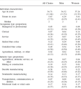
Table 1 presents descriptive statistics for the data analyzed in this study, including
Table 1
Summary Statistics for Wisconsin 1989–1990 Injuries with One or More Weeks of Lost Time
All Claims Men Women
Individual characteristics
Age in years 36.71 36.32 37.24
(11.66) (11.51) (11.91)
Tenure in years 5.87 6.29 5.01
(7.72) (8.25) (6.41)
Median 2 2 2
Occupation type (proportion)
Managerial or professional 0.05 0.03 0.09
(0.21) (0.16) (0.28)
Clerical 0.07 0.04 0.14
(0.26) (0.19) (0.35)
Service 0.15 0.07 0.29
(0.35) (0.26) (0.45)
Skilled blue collar 0.22 0.29 0.08
(0.41) (0.46) (0.26)
Unskilled blue collar 0.49 0.54 0.39
(0.50) (0.50) (0.49) Agricultural, military, or other 0.02 0.02 0.01
(0.13) (0.15) (0.09) Industry type (proportion)
Agricultural, domestic service, or 0.06 0.07 0.04
other (0.23) (0.25) (0.20)
Mining or construction 0.10 0.15 0.01
(0.30) (0.35) (0.07)
Durable manufacturing 0.28 0.31 0.23
(0.45) (0.46) (0.42)
Nondurable manufacturing 0.14 0.13 0.17
(0.35) (0.33) (0.37) Transportation, communication, or 0.07 0.09 0.02
utilities (0.25) (0.28) (0.15)
Table 1(continued)
All Claims Men Women
Finance, insurance, real estate, or 0.18 0.10 0.36
other services (0.39) (0.30) (0.48)
Employer characteristics
Number of employees 1,169 989 1,531
(2,324) (2,105) (2,675)
Median 237 162 421
Proportion of employees in firms 0.24 0.30 0.12 with 50 or fewer employees (0.43) (0.46) (0.32)
Proportion in public sector 0.10 0.08 0.12
(0.29) (0.28) (0.33)
Head, neck, or back 0.32 0.32 0.32
(0.46) (0.46) (0.47)
Back only 0.29 0.29 0.29
(0.45) (0.45) (0.45)
Upper extremities 0.28 0.25 0.33
(0.45) (0.43) (0.47)
Carpal tunnel syndrome 0.04 0.02 0.08
(0.20) (0.15) (0.27) Trunk, multiple, or different injuries 0.23 0.23 0.23
(0.42) (0.42) (0.42)
Lower extremities 0.18 0.21 0.13
(0.38) (0.40) (0.33) Claim characteristics
Proportion with permanent partial 0.18 0.19 0.17
disability (0.39) (0.39) (0.37)
Proportion with only temporary total 0.78 0.78 0.79
disability (0.41) (0.42) (0.41)
Proportion of claims compromised 0.04 0.03 0.05 (0.19) (0.18) (0.21) Earnings and employment
Pretax earnings one quarter before $5,499 $6,179 $4,129
injury ($3,420) ($3,547) ($2,666)
Median $5,112 $6,015 $3,736
Frequency of pre-injury employer 0.09 0.09 0.08
change (0.15) (0.16) (0.15)
Proportion changing employer after 0.17 0.18 0.16
injury (0.44) (0.45) (0.43)
Total number of observations 54,309 36,283 18,026
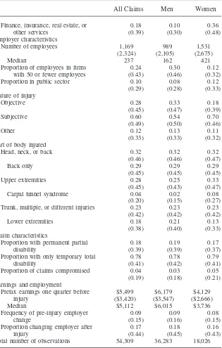
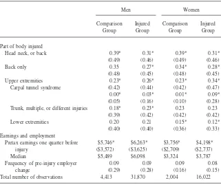
Figure 1
Changes in Quarterly Earnings Relative to Comparison Group
median values where distributions are skewed. On average, the workers we study were 36 years old and had six years of tenure with the pre-injury employer. Almost half were unskilled blue-collar workers. Only 24 percent were employed in firms with fewer than 50 employees and 10 percent were employed in the public sector. The most frequent injuries were back injuries (29 percent), incurred equally often by men and women. Men were slightly younger, had longer tenure and higher earn-ings, were more often blue-collar, and were more likely to be in mining, construction or durable manufacturing industries and in smaller firms. Women were more likely to have service, clerical, and managerial or professional jobs, be in the service sector or nondurable manufacturing and have upper-extremity injuries and, in specific, car-pal tunnel syndrome.
Figure 1 presents our first look at average differences between quarterly changes in earnings of injured workers3and in the comparison group. It represents difference-in-differences calculations of earnings, based on our raw data and therefore unad-justed for covariates.4We impute zero quarterly earnings in quarters for which no employer reports earnings for a person in our sample. The horizontal line at zero is the baseline, that is, the changes in earnings of the comparison group relative to the pre-injury quarter. In fact, we assume, for the moment, that the eight-to-ten day group experienced no losses.
3. For simplicity of exposition, we will refer to workers not in the comparison group as ‘‘injured workers,’’ although those in the comparison group had short-term injuries.
4. To create Figure 1, we generate changes in earnings as: [(YIt⫺Y10)⫺(YCt⫺YC0)]/Y10], whereyis
Figure 1 shows that, in the first two quarters after injury, men experience an aver-age percentaver-age loss in earnings relative to the comparison group that is about the same as for women. Yet, the unadjusted means suggest that over the next 3 1/2 years, men lost an average of 8.3 percent of pre-injury earnings while women lost 10.1 percent—about 1/4 higher than men. Figure 1 motivated this study and also helped us to specify the statistical model.
III. Methods
A. Basic Model of Earnings
We define injury-related lost earnings as the difference between workers’ actual post-injury earnings and what they would have earned if they had not been injured. We call theseobserved injured earningsanduninjured earningsrespectively. Of course, we do not observe uninjured earnings but must estimate them from data that we do observe. This estimation problem is parallel to those addressed by literature on nonexperimental program evaluation, where there is a substantial literature on esti-mating the impact of (for example) public-sector training programs. Here, the ‘‘treat-ment’’ is the injury, not a training program and the comparison group should ideally consist of workers who have not suffered the injury.
If we observe worker ibefore and after injury, we can write the model of that worker’s earnings as:
(1) yi⫽α1i⫹γt⫹Xi∗(α2⫹β1T)⫹εi
whereyis earnings,α1iis an individual-specific fixed effect,γtis a time-specific fixed effect capturing general economic conditions affecting all workers,T⫽0 before the
injury andT⫽1 after the injury, and X
i is a vector of observed and unobserved covariates. As long as noninjury factors do not affect the earnings path differentially in the pre-injury and post-injury periods, Equation 1 is a reasonable framework within which to estimate losses, withβ1measuring the impact of the injury on earn-ings.
However, because of the way our data were collected, even uninjured earnings are affected by their timing relative to the date of injury. This occurs because we assembled the data for people with a workplace injury in a given quarter. Because (by definition) 100 percent of people injured at work must have been employed when they were injured, employment rates will generally be lower in quarters before and after the injury, rising as the date of injury approaches and falling after the injury. This data-collection artifact would make it look as if losses occurred even for people whose earnings were unaffected by their injuries. As a consequence, the estimates of losses based on Equation 1 would be biased away from zero.
This is the type of situation that the difference-in-differences approach is designed to handle. Because it compares post-injury changes in earnings of the injured with changes in a suitably chosen uninjured comparison population, it can produce unbi-ased estimates of the impact of injuries under suitable conditions. This approach can be summarized by representing earnings as:
(1a) yi⫽α1i⫹γ
HereI⫽1 for the injured group andI⫽0 otherwise. The impact on the comparison
group’s uninjured earnings of measured and unmeasured factors is captured byα2. Differences in uninjured earnings between the injured and comparison groups are measured byα3.β1captures the data-collection artifact just described, andβ2 mea-sures the average effect of injury on earnings.
B. Selection Issues
The specification in Equation 1a describes the earnings of both injured and uninjured workers under fairly general conditions. It allows us to calculate expected losses for groups of workers with specific characteristics,Xiin each post-injury quarter. How-ever, this specification will provide unbiased estimates of losses if there is selection only on observable covariates (Rubin 1974), that is {γi1,γi0 Ii}|Xi(where indi-cates independence), or:
(2) E(yij|Xi,Ii⫽1)⫽E(yij|Xi,Ii⫽0),j⫽0,1
If Equation 2 holds, earnings and the probability of injury are independent after accounting for observable covariates, and there is no selection problem. However, there are several reasons that selection on unobservables might occur and therefore to expect a simple OLS model to provide biased estimates. For example, if safety is a normal good, then, ceteris paribus, the most productive (and highest wage) work-ers will have fewer injuries. On the other hand, for workwork-ers with the same human capital, compensating differentials can cause higher wages in more hazardous condi-tions. Reporting of injuries also maybe related to wages with low wage employees possibly more willing to report injury because of their higher income replacement rates associated with workers’ compensation benefits or because they are less likely to be covered by medical or disability insurance.5
Even when selection is on both observable and unobservable covariates, a differ-ence-in-differences estimator can identify the average treatment effect. If the unob-servables have effects that are additive, the same for injured and uninjured workers, and the same in the pre- and post-treatment periods, then the difference-in-differ-ences estimate will remove their impact and provide unbiased estimates of the impact of injuries (Imbens, Liebman, and Eissa 1997).
Still, there may be situations in which unobserved factors affect not only earnings levels but also both the growth of uninjured earnings and the probability of injury. For example, a poor employer-employee relationship could lead both to lower earn-ings growth and a higher probability of injury. Likewise, less-motivated workers may experience lower growth in earnings and may also be less careful and therefore more likely to have a serious injury. This is reflected by the coefficientα4in Equation 1b.
(1b) yi⫽α1i⫹γt⫹Xi∗(α2⫹α3∗I⫹α4t∗I⫹β1T⫹β2T∗I)⫹εi
This selection effect induces dependence between the trend in earnings and the prob-ability of injury based in part on unobservable factors, and it therefore produces selection on unobservable covariates. This, in turn, will cause bias in OLS estimates
of Equation 1b. But differencing the observations transforms the termα4ttoα4. That is, in the differenced form, the time trend term is transformed into a constant. Again, if the time trend (α4) is additive and the same in the pre-injury and post-injury periods, differencing will have eliminated this type of selection on unobservables and the difference-in-differences estimator will no longer be biased (Imbens, Lieb-man, and Eissa 1997).
C. The Comparison Group
We choose for a comparison group workers with short-duration injuries. These work-ers meet three criteria: (1) they had a single workplace injury from April 1, 1989 through September 30, 1990 and no subsequent injuries through 1993, (2) they lost eight to ten days from work and then returned,6and (3) they received no permanent disability payments.
Because workers’ compensation data provide information on several important personal characteristics, including gender, age, occupation, and job tenure, we can condition our estimates on these covariates. The matched unemployment insurance data allow us to condition on other factors, including industry, employer size, and workers’ pre-injury employment patterns.
We considered using uninjured workers as a comparison group, but our source of data on uninjured workers, the unemployment compensation wage files, does not provide information about gender (as well as age, occupation, and tenure). Because this information is critical to a study of gender discrimination, uninjured workers are problematic as a comparison group for this study. In addition, we expect that workers with short-term injuries are more like other injured workers on both ob-served and unobob-served characteristics than are uninjured workers.
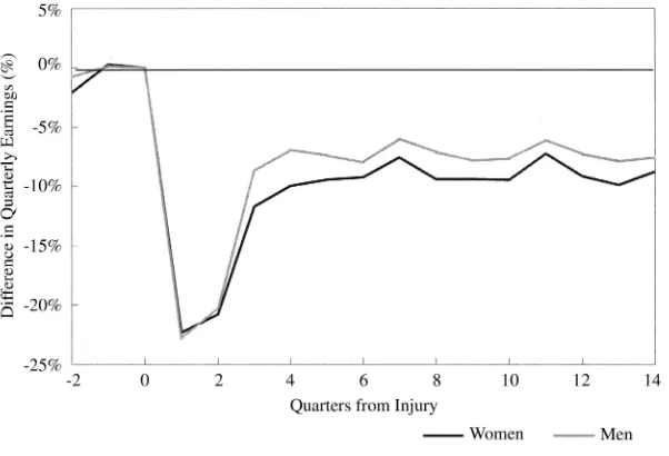
Table 2 presents for male and female workers the distribution of worker, employer, and injury characteristics for the comparison group and workers with longer-term injuries by gender. Workers in the comparison group tend to be younger, have less tenure, and earn less than those in the injured group. Occupation distribution is gener-ally similar between the two groups, although the comparison group for women has more service workers and fewer unskilled blue-collar workers. Workers in the comparison group are also more likely to be in wholesale, retail, or service industries, less likely to be in durable manufacturing, and less likely to work in larger firms.
These differences between the comparison group and the injured group suggest that there is selection into the injured population. However, when we estimate losses controlling for observed covariates, the trend in earnings of the injured group closely tracks the trend of the comparison group in the pre-injury period. This suggests that selection is predominately based on observed covariates.
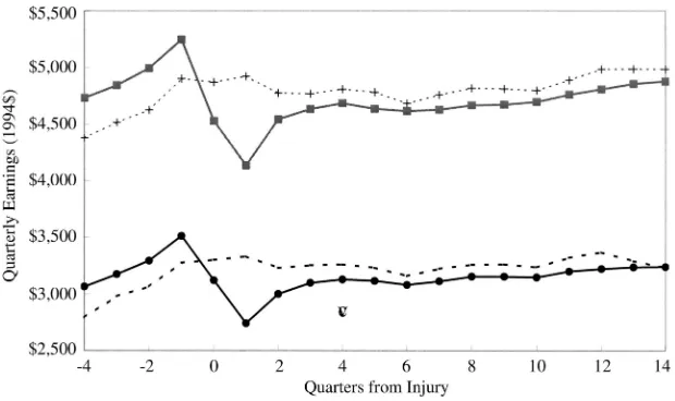
Figure 2 is based on our raw data and displays quarterly earnings in both the pre-injury and post-pre-injury periods. For both male and female workers, it shows that the younger, lower-tenure comparison group workers have lower average wages than
Table 2
Summary of Statistics for Wisconsin 1989–1990 Injuries: Comparison and Injured Groups
Men Women
Comparison Injured Comparison Injured
Group Group Group Group
Individual characteristics
Age in years 34.48* 36.59* 35.44* 37.46*
(11.76) (11.46) (11.91) (11.82)
Tenure in years 5.52* 6.42* 4.49* 5.09*
(7.62) (8.35) (6.09) (6.46)
Median 2 2 1 2
Occupation type (proportion)
Managerial or professional 0.03 0.03 0.11* 0.09*
(0.16) (0.16) (0.31) (0.28)
Clerical 0.04 0.04 0.17 0.14
(0.20) (0.19) (0.37) (0.35)
Service 0.09* 0.07* 0.35* 0.28*
(0.29) (0.26) (0.48) (0.45)
Skilled blue collar 0.29 0.29 0.06 0.08
(0.45) (0.46) (0.24) (0.27)
Unskilled blue collar 0.52 0.55 0.30* 0.40*
(0.50) (0.50) (0.46) (0.49)
Agricultural, military, or other 0.03* 0.02* 0.01 0.01
(0.16) (0.15) (0.09) (0.09)
Industry type (proportion)
Agricultural, domestic service, or other 0.07 0.07 0.06 0.05
(0.26) (0.25) (0.24) (0.22)
Mining or construction 0.14 0.15 0.01 0.01
(0.35) (0.36) (0.07) (0.08)
Durable manufacturing 0.28* 0.32* 0.17* 0.24*
(0.45) (0.47) (0.38) (0.42)
Nondurable manufacturing 0.12 0.13 0.15* 0.18*
(0.32) (0.33) (0.36) (0.38)
Transportation, communication, or 0.08 0.09 0.02 0.02
utilities (0.28) (0.29) (0.13) (0.15)
Wholesale trade or retail sales 0.19* 0.16* 0.20* 0.17*
(0.39) (0.37) (0.40) (0.37)
Finance, insurance, real estate, or other 0.12* 0.10* 0.39* 0.34*
services (0.32) (0.30) (0.49) (0.47)
Employer characteristics
Number of employees 902 1,001 1,428 1,548
(2,108) (2,105) (2,671) (2,678)
Median 141 166 359 430
Proportion of employees in firms with 0.30 0.29 0.13 0.12
50 or fewer employees (0.46) (0.45) (0.34) (0.32)
Proportion in public sector 0.09* 0.08* 0.14* 0.11
Table 2(continued)
Men Women
Comparison Injured Comparison Injured
Group Group Group Group
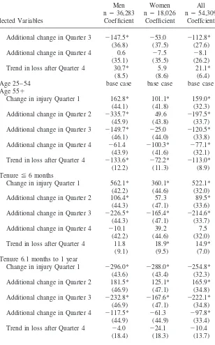
Part of body injured
Head neck, or back 0.39* 0.31* 0.39* 0.31*
(0.49) (0.46) (0.49) (0.46)
Back only 0.35 0.27* 0.34* 0.28*
(0.48) (0.45) (0.48) (0.45)
Upper extremities 0.23* 0.26* 0.23* 0.34*
Carpal tunnel syndrome (0.42) (0.44) (0.42) (0.47)
0.00* 0.03* 0.01* 0.09*
(0.05) (0.16) (0.10) (0.28)
Trunk, multiple, or different injuries 0.18* 0.23* 0.23 0.23
(0.39) (0.42) (0.42) (0.42)
Lower extremities 0.20 0.21 0.15* 0.12*
(0.40) (0.40) (0.36) (0.33)
Earnings and employment
Pretax earnings one quarter before $5,746* $6,263* $3,756* $4,198*
injury ($3,572) ($3,625) ($2,709) ($2,737)
Median $5,489 $6,098 $3,324 $3,787
Frequency of pre-injury employer 0.09 0.09 0.09 0.08
change (0.29) (0.28) (0.16) (0.15)
Total number of observations 4,413 31,870 2,004 16,022
* Difference between comparison and injured groups significant,p⬍.05
Note: Standard deviations are in parentheses. Statistical analysis is based on these data.
injured workers. Immediately post-injury, the wages of the injured workers fall below those of the comparison group. Injured workers’ earnings then rise, but re-main below the level of the comparison group. Note that the trend in earnings in both the pre-injury period and in the period beginning two to three quarters after injury is similar for both groups. However, the pre-injury difference in earnings implies that it would be inappropriate to use means unadjusted for covariates to estimate losses.
D. The Final Specification
Figure 2
Average Earnings, Control and Injured Group, Wisconsin Injuries, 1989–1990
(3) yi⫽α
1i⫹γt⫹α2X*i ⫹α3Ii⫹α4Ii∗t⫹
冱
k⫽0,5δk∗Fk
⫹
冱
k⫽1,5
δkI(Fk∗Ii∗Xi)⫹
冱
k⫽0,5ηk(Hk∗Ji)⫹εi
In Equation 3, the independent variable is earnings, not log (earnings) because the substantial number of periods with zero earnings would make estimation of a log (earnings) panel model problematic. The subscriptirefers to the individual worker andtrepresents the calendar quarter (for example, the first quarter of 1992). Quar-terly time dummies,γt, capture economic conditions affecting all workers in a given period.Fk(k⫽1,4) are dummy variables for the injury quarter and the three follow-ing quarters, each equal to zero before the quarter of interest and one durfollow-ing and after; andF5is the trend in earnings following this period.7Fkis the marginal impact of the injury in each quarter, so the impact of injury on wages in a given quarter is the sum of theFkfor that quarter and the preceding ones. The first line of the Equation 3 captures impacts of noninjury factors on earnings, and the second line captures the impacts of injuries. The termsα3Iiandα4Ii ∗ t(wheret is a time trend) capture respectively any difference in the mean and trend of pre-injury earnings between
7. Where q is the quarter relative to injury (q⫽0 in the quarter of injury), these variables are defined
as:
F0⫽
qifq⬍0,⫽0 otherwise
Fk⫽1 ifq⬎ ⫽k⫺1,⫽0 otherwise
F5⫽
the comparison group and the injured group. In addition, the terms∑k⫽0,5δk∗Fkare included to estimate common time-from-injury effects for all individuals. We need to estimate the coefficients of these terms to take into account an artifact of our data, which we collected for people with a workplace injury in a given quarter. As dis-cussed above, because 100 percent of this group must have been employed in the quarter of injury, employment rates will be lower in quarters before and after the injury, even if people lost no time from work because of their injuries. This data-collection artifact makes the use of a comparison group essential.
In the first line of Equation 3,X*i is a vector of observed fixed and time-varying individual characteristics that we would expect to affect earnings. This vector is composed ofage,age2,age3,age4; job tenure at the time of the injury (⬉6 months, 6.1 months to 1 year, 1.1 to 5 years, 5.1 to 10 years, greater than ten years; two-digit SIC dummies; one-two-digit Census occupational categories; log (number of the employees of the firm at the time of the injury); stability of pre-injury earnings (coefficient of variation of quarterly earnings); and frequency of pre-injury change of employer (number of changes divided by total changes possible for the observed pre-injury period). Except for age and employer size, all variables inX*i are inter-acted with a pre-injury trend and a post-injury trend.
The second line of Equation 3 captures the injury-related drop, recovery, and long-term trend in earnings. It includes an interaction of injury status with the five post-injury time-dummy or trend variablesFk. We allow this interaction to vary withXi, a vector of worker, employer, job, and injury characteristics (which may not be the same asX*i).Xiincludes: age at injury category (less than 25, 25–54, at least 55), employment size category (1–50, 51–250, 251–1,000, and more than 1,000 employ-ees), tenure category, two-digit industry, two-digit Census occupation, stability of pre-injury earnings, frequency of pre-injury employer change, and back and carpal tunnel injuries. It differs fromX*i essentially by including variables measured only at the time of injury. For example,X*i includes age in the current quarter and time trends for earnings by occupation, industry, and tenure, whileXiincludes age in the quarter of injury and no time trends.
Finally, about 30 percent of workers in our sample had more than one injury during the study period (that is, by the end of 1993). The model we use also accounts for the effects of injuries subsequent to the initial one with the term∑k⫽0,5(Hk∗Ji), whereJindicates a second injury. TheHkare parallel to theFk, but refer to periods relative to the second injury.
E. Estimates of Losses
We estimate our final earnings model (Equation 3) for men and women separately and together, based on our unbalanced panel. We note that if the error term is corre-lated across individuals, the resulting OLS estimator will be inefficient and the esti-mated variances will be biased. But such bias can be removed by estimating the difference-in-differences model using GLS. In fact, we find substantial first-order autocorrelation in earnings, so we have estimated the first-differences version of Equation 3 using GLS and allowing for first-order autocorrelaton.8
8. The estimates of first order autocorrelation in the first-difference specification areρ⫽ ⫺0.33 for men
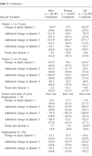
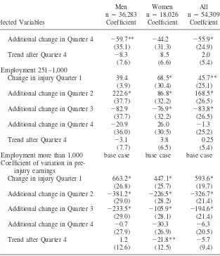
Table 3 presents regression coefficients that measure average post-injury earnings relative to the comparison group for the base case, which is a 25–54 year old un-skilled blue-collar worker who had been working at least 10 years at a firm in durable manufacturing with more than 1,000 workers, whose earnings were constant during the observed pre-injury period, and whose injury did not involve low back pain or carpal tunnel syndrome.
Among men, the estimate of pre-injury earnings growth for the comparison group is $21 per quarter less than that for other injured workers (p⫽0.07). For women,
Table 3
GLS Estimates of Quarterly Earnings, First Differences, Lost-Time Injuries in Wisconsin, 1989–1990
Men Women All
n⫽36,283 n⫽18,026 n⫽54,309
Selected Variables Coefficient Coefficient Coeffcient
Variables-affecting earnings (α1)
Constant (trend) ⫺5.9 ⫺108.4 ⫺26.6
(26.1) (25.1) (19.2)
Age2 0.70* 0.59* 0.55*
(0.24) (0.22) (0.17)
Age3 ⫺0.105* ⫺0.068* ⫺0.083*
(0.020) (0.018) (0.015)
Female — — ⫺5.2
(3.1) Injury impact (δkI)
Pre-injury trend 21.9** 2.3 14.7
(12.1) (12.4) (9.1)
Loss in injury Quarter 1 ⫺1497.1* ⫺1025.0* ⫺1372.9*
(48.9) (51.4) (36.8)
Additional loss in Quarter 2 ⫺459.8* ⫺444.8* ⫺460.5*
(51.6) (54.6) (39.0)
Recovery in Quarter 3 1153.0* 684.5* 1012.5*
(51.6) (54.7) (39.0)
Recovery in Quarter 4 112.6* 107.3* 107.4*
(49.3) (51.9) (37.2)
Trend in loss after Quarter 4 34.8* 55.5* 36.4*
(15.3) (17.0) (11.8)
Injury impacts of selected charac-teristics (δKI)
Age 15–24
Change in injury Quarter 1 280.4* 164.8* 236.0*
(35.3) (35.7) (26.4)
Additional change in Quarter 2 272.2* 44.1 196.2*
Table 3(continued)
Men Women All
n⫽36,283 n⫽18,026 n⫽54,309
Selected Variables Coefficient Coefficient Coeffcient
Additional change in Quarter 3 ⫺147.5* ⫺53.0 ⫺112.8*
(36.8) (37.5) (27.6)
Additional change in Quarter 4 0.6 ⫺7.5 ⫺8.1
(35.1) (35.5) (26.2)
Trend in loss after Quarter 4 30.7* 5.9 21.1*
(8.5) (8.6) (6.4)
Age 25–54 base case base case base case
Age 55⫹
Change in injury Quarter 1 162.8* 101.1* 159.0*
(44.1) (41.8) (32.3)
Additional change in Quarter 2 ⫺335.7* 49.6 ⫺197.5*
(45.9) (43.8) (33.7)
Additional change in Quarter 3 ⫺149.7* ⫺25.0 ⫺120.5*
(46.1) (44.0) (33.8)
Additional change in Quarter 4 ⫺61.4 ⫺100.3* ⫺77.1*
(43.9) (41.6) (32.1)
Trend in loss after Quarter 4 ⫺133.6* ⫺72.2* ⫺113.0*
(12.2) (11.3) (8.9)
Tenure⬉6 months
Change in injury Quarter 1 562.1* 360.1* 522.1*
(42.2) (44.6) (32.0)
Additional change in Quarter 2 106.4* 57.3 89.5*
(44.3) (47.1) (33.6)
Additional change in Quarter 3 ⫺226.5* ⫺165.4* ⫺214.6*
(44.3) (47.1) (33.7)
Additional change in Quarter 4 ⫺10.1 39.2 7.5
(42.2) (44.6) (32.0)
Trend in loss after Quarter 4 11.8 18.9* 14.9*
(9.1) (9.5) (7.0)
Tenure 6.1 months to 1 year
Change in injury Quarter 1 ⫺296.0* ⫺288.0* ⫺254.8*
(43.6) (43.4) (32.3)
Additional change in Quarter 2 181.5* 125.1* 165.9*
(46.9) (47.1) (34.8)
Additional change in Quarter 3 ⫺232.8* ⫺167.6* ⫺222.1*
(46.9) (47.1) (34.8)
Additional change in Quarter 4 ⫺117.5* ⫺61.3 ⫺97.8*
(44.9) (44.9) (33.4)
Trend in loss after Quarter 4 ⫺4.0 ⫺24.1 ⫺10.4
Table 3(continued)
Men Women All
n⫽36,283 n⫽18,026 n⫽54,309
Selected Variables Coefficient Coefficient Coeffcient
Tenure 1.1 to 5 years
Change in injury Quarter 1 70.9** 57.3 101.9*
(38.8) (40.2) (29.2)
Additional change in Quarter 2 132.3* ⫺29.4 78.7*
(42.1) (44.1) (31.8)
Additional change in Quarter 3 ⫺231.5* ⫺181.6* ⫺277.1*
(42.1) (44.2) (31.8)
Additional change in Quarter 4 ⫺30.3 ⫺50.3 ⫺35.2
(40.4) (42.2) (30.5)
Trend after Quarter 4 ⫺2.8 ⫺29.0 ⫺8.8
(18.2) (19.3) (13.8)
Tenure 5.1 to 10 years
Change in injury Quarter 1 119.2* 76.1 145.6*
(46.6) (45.2) (34.2)
Additional change in Quarter 2 133.3* ⫺111.7* 44.3
(50.9) (50.0) (37.6)
Additional change in Quarter 3 ⫺196.4* ⫺55.8 ⫺162.9*
(50.9) (50.0) (37.6)
Additional change in Quarter 4 65.1 24.3 48.0
(48.9) (47.9) (36.1)
Trend after Quarter 4 1.6 ⫺33.1 ⫺9.9
(23.4) (23.3) (17.5)
Tenure more than 10 years base case base case base case Employment⬍50
Change in injury Quarter 1 32.6 17.3 ⫺1.9
(36.9) (41.4) (27.7)
Additional change in Quarter 2 199.3* 217.0* 209.4*
(38.9) (43.9) (29.1)
Additional change in Quarter 3 ⫺79.2* ⫺193.3* ⫺100.0*
(38.9) (43.9) (29.1)
Additional change in Quarter 4 ⫺98.4* ⫺35.2 ⫺92.3*
(37.0) (41.5) (27.7)
Trend after Quarter 4 7.7 7.6 10.0**
(8.0) (8.8) (6.0)
Employment 51–250
Change in injury Quarter 1 ⫺13.1 41.5 ⫺19.4
(34.5) (31.2) (24.9)
Additional change in Quarter 2 152.6* 110.3* 145.4*
(36.8) (33.0) (26.2)
Additional change in Quarter 3 ⫺52.2 ⫺111.4* ⫺71.2*
Table 3(continued)
Men Women All
n⫽36,283 n⫽18,026 n⫽54,309
Selected Variables Coefficient Coefficient Coeffcient
Additional change in Quarter 4 ⫺59.7** ⫺44.2 ⫺55.9*
(35.1) (31.3) (24.9)
Trend after Quarter 4 ⫺8.3 8.5 2.0
(7.6) (6.6) (5.4)
Employment 251–1,000
Change in injury Quarter 1 39.4 68.5* 45.7**
(3.9) (30.4) (25.1)
Additional change in Quarter 2 222.6* 86.8* 168.5*
(37.7) (32.2) (26.5)
Additional change in Quarter 3 ⫺82.9 ⫺76.9* ⫺83.8*
(37.7) (32.2) (26.5)
Additional change in Quarter 4 ⫺20.9 26.0 ⫺1.3
(36.0) (30.5) (25.2)
Trend after Quarter 4 ⫺3.1 3.8 0.25
(7.7) (6.5) (5.4)
Employment more than 1,000 base case base case base case Coefficient of variation in
pre-injury earnings
Change in injury Quarter 1 663.2* 447.1* 593.6*
(26.8) (25.7) (19.7)
Additional change in Quarter 2 ⫺381.2* ⫺226.5* ⫺326.7*
(29.0) (28.2) (21.4)
Additional change in Quarter 3 ⫺233.5* ⫺105.9* ⫺194.6*
(29.0) (28.1) (21.4)
Additional change in Quarter 4 ⫺0.7 ⫺30.3 ⫺6.3
(27.9) (26.9) (20.5)
Trend after Quarter 4 1.2 ⫺21.8** ⫺5.7
(12.6) (12.5) (9.4)
* Significant,p⬍.05
** Significant,p⬍.10
Note: The omitted categories used imply that the estimates of injury impacts displayed in this table are for the base case of a 25–54 year old unskilled blue-collar worker in a durable manufacturing industry with ten years of tenure in a firm with over 1,000 employees. This worker had constant earnings in the pre-injury period and the injury did not involve low back pain or carpal tunnel syndrome. Each person is observed for 24 time periods. Because we use first differences, this results in 23 observations per person, or 1,249,107 observations overall. The estimations also included coefficients representing changes in in-come related to a second injury and dummy variables for each time period (with the first observed quarter omitted). We omit from this table the coefficients of variables affecting uninjured earnings: age2, age3; job
tenure at the time of the injury (ⱕ6 months, 6.1 months to 1 year, 1.1 to 5 years, 5.1 to 10 years, greater
Table 4
Estimated Average Percentage of Earnings Lost, Men and Women Injured at Work
Quarters from Injury Men’s Losses Women’s Losses
1–2 21.2% 21.7%
3–16 6.5% 9.2%
1–16 8.2% 10.7%
the equivalent estimate is $2 per quarter more (p⬎ 0.85). In neither case is the
difference large. This implies that we cannot reject the hypothesis of equality in the trend of uninjured earnings between the comparison group and the injured group of women; for men, the difference is on the margin of statistical significance, although the amount is not large. Similar pre-injury earnings growth suggests that the choice of comparison group is reasonable.
Given this estimation of Equation 3, we calculate expected uninjured earnings for each individual and time period by setting to zero the coefficients of the interac-tions measuring the impact of injuries (δkI⫽0 andηk⫽0). Next, for each person in the sample, we calculate expected losses, that is, actual earnings minus expected uninjured earnings. To obtain total losses, we also add each worker’s average pre-injury daily wage multiplied by nine days, the average duration of lost time in the comparison group. Then, the expected average percentage of earnings lost is ex-pected losses divided by exex-pected uninjured earnings. They are displayed in Table 4 and Figure 3.9
The results are consistent with the pattern we had detected originally in the raw data in Figure 1. In Table 4 and Figure 3, women’s losses in the quarter of injury and in the next quarter average 21.7 percent of expected uninjured earnings, a little more than men’s, which average 21.2 percent. However, shortly after the injury, the disparity increases sharply, and women’s losses become greater than men’s, averag-ing 2.7 percentage points higher than men’s for the remainder of the observed period (women lose an average of 9.2 percent of earnings, while men lose only 6.5 percent). From another perspective, women’s proportionate losses average 42 percent higher than men’s over this period.
Figure 3
Estimated Percent of Earnings Lost, Wisconsin Injuries, 1989–1990
IV. The Impact of Differential Characteristics on
Gender Differences in Losses
Disparities in the proportionate losses of men and women could come about as a result of different personal, employer, or job characteristic. For example, larger employers may find it easier to provide a period of light-duty work for workers who haven’t fully recovered from their injuries and women could be less represented in large firms (although this is not the case in our data). Also, some gender differences in losses might be caused by differences in occupational distribution. It is possible (although unlikely, given the gender distribution of occupations) that women’s jobs are more physically demanding, so they might find it harder to continue working after they are injured. In this case, they could lose wages related to occupation-specific human capital. Alternatively, women might return to jobs that pay smaller compensating differentials, and this reduction might be greater than that experienced by men. These factors would be captured by a statistical approach that took occupa-tion and other observed characteristics into account, unless there were important gender differences along these dimensions within occupational categories.
work. Women are paid less, on average, and yet may have an opportunity cost of going back to work that is at least as high as for men. It is also possible that women are more responsive to changes in wages (Kahn and Griesinger 1989; Sicherman 1996; Galizzi 2001). As a result, once they realize that the injury is leading them to jobs with lower wages or lower wage growth, they may be more likely to take longer to return to work or to leave the labor force.
Alternatively, on the demand side of the market we have already noted that em-ployers may be more willing to employ (or reemploy) men after their injuries because of discriminatory beliefs or because employers can obtain better predictions of men’s skills or mobility behaviors. Also, women may be easier to replace, once they are off work because of an injury, because of their average lower accumulation of job specific human capital. At the same time, it is possible that women’s jobs are more flexible, allowing women to work fewer hours post injury.
A. Wage Decomposition
As a first step toward understanding gender disparities in losses, we examine the extent to which observed personal, job, employer, and injury characteristics account for these disparities. To do this, we apply an extension of the Oaxaca-Blinder decom-position (Oaxaca 1973; Blinder 1973).
Neumark’s (1998) general version of the decomposition can be written as:
(4) W¯m⫺W¯f⫽(X¯m⫺X¯f)b⫹[X¯m(bm⫺b)⫺X¯f(bf⫺b)]
WhereW¯mandW¯fare gender-specific average wages,X¯mandX¯fare vectors of aver-age characteristics,brepresents the nondiscriminatory wage structure referring to the pooled male-female labor force, whilebmandbfare gender-specific wage struc-tures. The first term in Equation 4 represents the portion of the male-female wage disparity that is due to differences in characteristics. The second term, in the square brackets, is the portion of wage differentials unexplained by differences in character-istics, and often is used to measure discrimination. The first part of the term in brackets represents the male advantage (‘‘nepotism’’) compared with the nondiscriminatory wage structure. Similarly the second part of that term represents the female disadvan-tage (‘‘discrimination’’). Although these and related measures often have been used as a measure of employer gender discrimination, they also could reflect gender differ-ences in worker responses to injury or the impact of unmeasured covariates.
We adapt the Oaxaca-Blinder-Neumark method to decompose injury related losses. Therefore, we apply it to injury-related losses estimated from Equation 3, and not to wages. We allow the loss coefficients to vary in the quarter of injury and in each of the four subsequent quarters and to have a long-term trend. Therefore, our new specification differs from Equation 4 in having the gender difference in losses as the dependent variable and in allowing losses to change with time after injury:
(4a) L¯mk⫺L¯fk⫽
冱
k⫽1,5 Fk{(X¯
mk ⫺X¯fk)bk⫹[X¯mk(bmk ⫺bk)⫺X¯fk(bfk⫺bk)]}
Here,Lkis the estimate of the injury-induced change in earnings in periodkrelative to the quarter of injury derived from the results of Table 3;X¯kis a vector of mean characteristics in periodk, andbkis a vector of coefficients for the periodkrelative to the injury. Of course, themandfsubscripts represent male and female. Variables without subscripts refer to the entire population. As in Equation 3, the impact of injury on wages in a given quarter is the sum of theFkfor that quarter and the preceding ones.
B. Results of Decomposition
Our original estimates of losses had shown that in the quarter of injury and in the following quarter, men’s and women’s percentage losses were very similar: both average a little more than 20 percent of expected uninjured earnings. Over the next three and a half years, however, women’s losses averaged 2.7 points more than men’s. We use the loss decomposition in a (4a) to determine the amount of the difference accounted for by gender disparities in characteristics (bk), calculating expected losses from the full-sample parameter estimates at the means of the co-variates for both men and women (Figure 4 and Table 5). During the first two
Figure 4
Table 5
Decomposition of Estimates of Gender Differences in Injury-Related Losses
Women’s Losses minus Men’s Losses
(percent of injured earnings)
Quarters from Injury
1–2 3–16
1. Male advantage due to characteristic 3.5% ⫺1.1%
2. Male advantage due to behavior ⫺0.8% 0.9%
3. Female advantage due to behavior 2.3% ⫺3.0%
4. Overall male advantage due to behavior (2.⫺3.) ⫺3.1% 4.0%a
5. Overall difference (1.⫹4.) 0.4% 2.8%a
a. Numbers do not sum exactly because of rounding.
quarters after injury, the full-sample (nondiscriminatory) parameter estimates generate men’s losses that are 3.5 points less than women’s (Table 5, Row 1). After this initial period, the result reverses and women’s expected nondiscrimin-atory losses average 1.1 points less than those of men. This suggests that, if there were no discrimination or gender differences in behavior, women would initially have lost more, but in the longer term they would have lost a smaller proportion of earnings.
Figure 5
Estimated Percent of Earnings Lost Men Injured in Wisconsin, 1989–1990
Figure 6
To test the hypothesis that characteristics alone explain the difference between the losses of men and of women, we calculate bootstrapped standard errors of the overall male advantage due to behavior in each period. We use 50 bootstrapped samples from the overall data to calculate the mean overall male advantage, which is our measure of women’s losses attributable to discrimination. For all quarters, the 95 percent confidence interval for the impact of behavior on proportionate earnings losses does not include zero. This leads us to reject the hypothesis that the observed disparity in long-term losses is caused only by differences in observed personal, employer, job, or injury characteristics.
V. The Impact of Nonemployment on Gender
Differences in Losses
Our next step consists in looking for alternative labor-market features that may cause the observed gender disparity in long-term losses. The first hypothesis we examine is that women and men differ in their employment patterns after injury. Our data can tell us whether individuals had positive covered earnings in each ob-served quarter, allowing us to measure the impact on losses caused by different post-injury employment patterns.
To do this, we estimate the impact of injury on the probability of employment (positive earnings) in each quarter with logistic regression, using the White-Huber adjustment (White 1980) to account for within-person correlation. These estimates use the same independent variables as the loss estimates (Equation 3). Hardware limitations prevent us from using more than 9,100 observations in the logistic regressions, so we randomly sampled men and women to get sample sizes under this limit. Selected coefficients from the logistic regressions are displayed in Table 6.
Table 6
Logistic Estimates of the Probability of Being Employed, Men and Women with Lost-Time Injuries
Change in quarter after injury, Quarter 2 ⫺0.94* ⫺1.78*
(0.37) (0.39)
Additional change in Quarter 3 0.97* 0.94*
(0.30) (0.33)
Additional change in Quarter 4 ⫺0.30 0.02
(0.22) (0.24)
Trend after Quarter 4 ⫺0.07 0.00
(0.03) (0.03)
Individual characteristics Age 15–24
Change in quarter after injury, Quarter 2 0.27* 0.11
(0.13) (0.13)
Additional change in Quarter 3 ⫺0.20* 0.13
(0.12) (0.10)
Additional change in Quarter 4 0.28* 0.10
(0.11) (0.12)
Trend after Quarter 4 0.02* ⫺0.01
(0.01) 0.01
Age 25–54 base case base case
Age 55⫹
Change in quarter after injury, Quarter 2 ⫺0.37* ⫺0.41*
(0.19) (0.18)
Additional change in Quarter 3 ⫺0.02 0.20
(0.16) (0.15)
Additional change in Quarter 4 0.13 ⫺0.39
(0.10) (0.12)
Trend after Quarter 4 ⫺0.04* ⫺0.03*
(0.01) (0.01)
Tenure⬉6 months
Change in quarter after injury Quarter 2 0.93* 1.03*
(0.27) (0.29)
Additional Change in Quarter 3 ⫺0.43* ⫺0.29
(0.20) (0.20)
Additional Change in Quarter 4 0.09 0.18
(0.16) (0.15)
Trend after Quarter 4 0.04 ⫺0.02
Table 6(continued)
Men Women
n⫽9,050 n⫽9,013
Tenure 6.1 months to 1 year
Change in quarter after injury Quarter 2 ⫺0.06 ⫺0.30
(0.28) (0.30)
Additional change in Quarter 3 ⫺0.39 ⫺0.38*
(0.21) (0.21)
Additional change in Quarter 4 0.06 0.16
(0.17) (0.15)
Trend after Quarter 4 0.12* 0.07*
(0.03) (0.03)
Tenure 1.1 to 5 years
Change in quarter after injury, Quarter 2 0.06 ⫺0.39
(0.30) (0.33)
Additional change in Quarter 3 ⫺0.02 ⫺0.09
(0.16) (0.22)
Additional change in Quarter 4 0.02 ⫺0.07
(0.17) (0.16)
Trend after Quarter 4 0.10* 0.01
(0.03) (0.03)
Tenure 5.1 to 10 years base case base case
Tenure more than 10 years
Change in quarter after injury (2) 0.34 0.34
(0.31) (0.38)
Additional change in Quarter 3 ⫺0.27 ⫺0.36
(0.23) (0.24)
Additional change in Quarter 4 0.04 0.25
(0.18) (0.17)
Trend after Quarter 4 0.07* 0.04*
(0.03) (0.03)
Wald X2(201) 11,091.84 10,824.81
* Significant,p⬍.05
Figure 7
Estimated Injury-Related Nonemployment Workers Injured in Wisconsin, 1989– 1990
VI. Other Possible Explanations for Observed
Differences
In this section, we briefly consider alternate explanations of the ob-served gender disparities in losses that do not rely on discrimination, providing evi-dence where we can. There is marginal support for one of these explanations: Women reduce their hours of work more than men do. The evidence generally does not support the other hypotheses.
1. Hypothesis: Women’s injuries are more severe, causing greater long-term health consequences and, therefore, greater loss in earning capacity.
A telephone survey of a subsample of the study population that had back injuries (Galizzi, Boden, and Liu 1998) allows us to see whether there appear to be substantial gender-related differences in injury severity for a subset of workplace injuries. We compare measures of severity for the comparison group (eight to ten days’ lost time) with workers who received permanent partial disability benefits or at least four weeks of temporary disability benefits.10The most direct measures of injury severity in this survey are overnight hospitalization and surgery. By these measures, men’s injuries were more severe: 16 percent of men and 11 percent of women were hospitalized overnight. In addition, 26 percent of men and 21 percent of women had back surgery.
Table 7
Tobit Estimate of Physical Functioning of Injured Workers
Coefficient
Variable (n⫽1,179)
Constant 139.23*
(4.68)
Age ⫺0.80*
(0.10)
Female ⫺11.63*
(5.07)
Injured (comparison group⫽0) ⫺25.90*
(⫺8.08)
Injured * Female ⫺0.35
(5.74)
Note: The results are based on a sample of workers with back injuries. The dependent variable is the physical functioning subscale of the SF-36 instrument, with an allowable range of 0 to 100. A higher number indicates better physical functioning. Standard errors are in parentheses.
Less than 1 percent of men and women in the comparison group reported injury-related surgery, and less than 2 percent reported overnight hospitalization. The sur-vey also asked people to describe physical limitations related to ten common activi-ties, which compose the physical functioning subscale of the SF-36 Health Profile (Ware et al. 1993). Average current functional limitations reflect, in part, the impact of the injury. Physical functioning is scored between 0 and 100, where 100 represents no limitations. On average men in the comparison group scored 91.1 while women scored 85.5, a disparity similar to that in the overall U.S. population gender differ-ence in physical functioning scores of 5.7 points (Ware et al. 1993). We used a Tobit specification to regress the physical functioning score on age, a gender-effect dummy variable (representing noninjury related gender differences), an injury-effect dummy (capturing whether workers were in the comparison or in the injured group), and a gender-injury interaction, reflecting gender differences in injury severity (Table 7). The results show that, while women overall report greater limitations than men, injuries do not increase their reported limitations more than men’s. Once again, there is no evidence that women’s injuries are more severe than men’s.
2. Hypothesis: Women preferentially move from full-time to part-time jobs after injury, as they do after displacement (McCall 1997).
ap-proach, comparing changes in weekly hours in the comparison group to changes in the group with PPD benefits or at least four weeks of temporary disability benefits. Women in the latter group reduced their weekly work by 5.7 hours relative to the comparison group. This number is 5.5 for men (Table 8). Because men worked more hours than women did before they were injured, the reduction in hours averaged 14.7 percent (5.7/38.7) for women and 12.1 percent (5.5/45.4) for men—a differential of 2.6 percentage points. Combined with the 1.4 point gender differential in injury-related nonemployment, changes in hours could explain the difference in men’s and women’s losses.
However, several important covariates may influence this relationship. These in-clude the differential impact of injuries by occupation and industry. We control for these by regressing the ratio of post-injury hours to pre-injury hours on pre-injury hours, an injury dummy, sex, occupation, industry, firm size, and the interactions of these variables with the injury dummy. We test the hypothesis that the interaction of sex and injury is zero, that is, that women and men have the same injury-related percentage reduction in hours. The coefficient is 0.0005, withp⬎0.99.11
The role of reduced hours in the gender differential in losses is at this point incon-clusive. Our estimate is statistically insignificant, but we do not rule out the possibil-ity that differential changes in hours may explain part or all of the observed gender gap in injury-related losses that remains after accounting for nonemployment.
3. Hypothesis: Women are less attached to the labor force, so they more frequently withdraw from the labor force after they are injured.
Only about 3.1 percent of injured workers in our study did not return to work during the study period, and this group had fewer women (2.9 percent) than men (3.2 per-cent). To control for the impact of covariates, we estimate a multivariate logistic regression (dependent variable equal to one if the worker lacked earnings in all ob-served post-injury quarters). Age, tenure, industry, part of body injured, unemploy-ment rate, and employer size virtually completely account for the gender difference, leaving an insignificant difference between women and men (Table 9; female to male odds ratio⫽1.06,95 percent C.I.⫽0.93–1.22). This result is consistent with
a previous study, where we looked at the probability that injured workers were work-ing one year after the first return to work (Galizzi and Boden 1996). For men and women with the same personal and employer characteristics, women were slightly less likely to be working a year after the first return, but the estimated difference is well under one percentage point. Both findings suggest that long-term withdrawal from the labor force is unlikely to explain our findings.
4. Hypothesis: Women less frequently return to their pre-injury place of employment. Therefore, they lose any job specific human capital, and any return to the tenure they had accumulated with their pre-injury employers.
Among the workers we study, about the same proportion of men (84.7 percent) and women (86.7 percent) returned to the preinjury employer. Two years after the injury,
The
Journal
of
Human
Resources
Table 8
Percent Full-time and Weekly Hours Worked Before and After Injury
Men Women
Comparison Injured Comparison Injured
Group Group Difference Group Group Difference
Percent full time, pre-injury 94.3 96.7 2.4 72.5 81.0 8.5
Percent full time, latest job 95.0 84.4 ⫺10.6 67.8 53.8 ⫺14.0
Difference 0.7 ⫺12.3 ⫺13.0 ⫺4.7 ⫺27.2 ⫺22.5
Average hours, pre-injury 43.3 45.4 2.1 37.1 38.7 1.6
Average hours, latest job 43.5 40.1 ⫺3.4 36.0 31.9 ⫺4.1
Difference 0.1 ⫺5.3 ⫺5.5 ⫺1.1 ⫺6.8 ⫺5.7
Table 9
Estimates of the Probability of Never Working after Injury, Men and Women
Selected Variables n⫽54,309
Constant ⫺5.29*
(0.51) Individual characteristics
Age⬍25 ⫺0.33
(0.08)
Age 25–54 base case
Age 55⫹ 1.33*
(0.08)
Tenure⬉6 months 0.99*
(0.12)
Tenure 0.6–1 year 0.77*
(0.12)
Tenure 1.1–5 years 0.39*
(0.12)
Tenure 5.1–10 years 0.15
(0.14)
Tenure 10⫹years base case
Male base case
Female 0.05
(0.07) Employer characteristics
1–50 employees 0.54*
(0.10)
51–250 employees 0.40*
(0.09)
251–1,000 employees 0.09
(0.10)
1,000⫹employees base case
52.0 percent of men and 51.9 percent of women remained at the pre-injury employer; one year after that, these percentages were 45.1 and 44.0. Using logistic regression to estimate the probability of initially returning to work for the same employer while controlling for covariates (age, tenure, two-digit occupation, part of body injured, size, unemployment rate, weekly wage pre-injury earnings variation, and the fre-quency of pre-injury employer change), women with the same covariates as men appear to returnmorefrequently to the pre-injury employer (female-male odds ratio
⫽1.30, 95 percent C.I.⫽1.22–1.39). Because they return more frequently to the
pre-injury employer, it is unlikely that injured women more frequently lose specific human capital than do men.12(This finding also calls into question the hypothesis that pre-injury employers discriminate against injured women.)
5. Hypothesis: After the injury, women return to jobs that do not pay compensating wage differentials.
In one of the few studies looking at gender differences among injured workers, Hersch (1998) found that both men and woman are compensated for working in more risky jobs, and that occupational risk, and not industry risk, has a significant effect on women’s wages. But, the loss-decomposition results, which took occupa-tion into account, did not reduce the gender disparity in losses. Furthermore, as was just noted, women do not seem to change employer more often than men. Therefore, our data appear inconsistent with an explanation based on lost compensating wage differentials.
6. Hypothesis: Women are more likely than men to be reinjured, so employers reduce their wage offers to injured women relative to men.
Our data contain information about subsequent injuries over the period 1989–94. Only 35.2 percent of women in our sample experienced a subsequent workplace injury, compared with 40.4 percent of men. (However, this result is only suggestive because workers who are likely to be reinjured may have lower probabilities of post-injury employment and therefore have fewer injuries because they have less exposure to the risk of workplace injury.)13
7. Hypothesis: Women take longer to return to work, possibly because their replacement of losses by workers’ compensation benefits is greater or because the opportunity cost of working is greater.
A study of return to work in this same group of workers (Galizzi and Boden 1996) provides at best mixed evidence about this assertion. In this group, initial return to work averaged three days longer for men than for women, although women’s median time off work was seven days longer than men’s. We also estimated that workers’
12. Results available from the authors.