3
Algorithm Analysis
How long will it take to process the company payroll once we complete our planned merger? Should I buy a new payroll program from vendor X or vendor Y? If a particular program is slow, is it badly implemented or is it solving a hard problem?
Questions like these ask us to consider the difficulty of a problem, or the relative efficiency of two or more approaches to solving a problem.
This chapter introduces the motivation, basic notation, and fundamental tech- niques of algorithm analysis. We focus on a methodology known asasymptotic algorithm analysis, or simplyasymptotic analysis. Asymptotic analysis attempts to estimate the resource consumption of an algorithm. It allows us to compare the relative costs of two or more algorithms for solving the same problem. Asymptotic analysis also gives algorithm designers a tool for estimating whether a proposed solution is likely to meet the resource constraints for a problem before they imple- ment an actual program. After reading this chapter, you should understand
• the concept of a growth rate, the rate at which the cost of an algorithm grows as the size of its input grows;
• the concept of upper and lower bounds for a growth rate, and how to estimate these bounds for a simple program, algorithm, or problem; and
• the difference between the cost of an algorithm (or program) and the cost of a problem.
The chapter concludes with a brief discussion of the practical difficulties encoun- tered when empirically measuring the cost of a program, and some principles for code tuning to improve program efficiency.
3.1 Introduction
How do you compare two algorithms for solving some problem in terms of effi- ciency? One way is to implement both algorithms as computer programs and then 57
run them on a suitable range of inputs, measuring how much of the resources in question each program uses. This approach is often unsatisfactory for four reasons.
First, there is the effort involved in programming and testing two algorithms when at best you want to keep only one. Second, when empirically comparing two al- gorithms there is always the chance that one of the programs was “better written”
than the other, and that the relative qualities of the underlying algorithms are not truly represented by their implementations. This is especially likely to occur when the programmer has a bias regarding the algorithms. Third, the choice of empirical test cases might unfairly favor one algorithm. Fourth, you could find that even the better of the two algorithms does not fall within your resource budget. In that case you must begin the entire process again with yet another program implementing a new algorithm. But, how would you know if any algorithm can meet the resource budget? Perhaps the problem is simply too difficult for any implementation to be within budget.
These problems can often be avoided by using asymptotic analysis. Asymp- totic analysis measures the efficiency of an algorithm, or its implementation as a program, as the input size becomes large. It is actually an estimating technique and does not tell us anything about the relative merits of two programs where one is always “slightly faster” than the other. However, asymptotic analysis has proved useful to computer scientists who must determine if a particular algorithm is worth considering for implementation.
The critical resource for a program is most often its running time. However, you cannot pay attention to running time alone. You must also be concerned with other factors such as the space required to run the program (both main memory and disk space). Typically you will analyze thetimerequired for analgorithm(or the instantiation of an algorithm in the form of a program), and thespacerequired for adata structure.
Many factors affect the running time of a program. Some relate to the environ- ment in which the program is compiled and run. Such factors include the speed of the computer’s CPU, bus, and peripheral hardware. Competition with other users for the computer’s resources can make a program slow to a crawl. The program- ming language and the quality of code generated by a particular compiler can have a significant effect. The “coding efficiency” of the programmer who converts the algorithm to a program can have a tremendous impact as well.
If you need to get a program working within time and space constraints on a particular computer, all of these factors can be relevant. Yet, none of these factors address the differences between two algorithms or data structures. To be fair, pro- grams derived from two algorithms for solving the same problem should both be
compiled with the same compiler and run on the same computer under the same conditions. As much as possible, the same amount of care should be taken in the programming effort devoted to each program to make the implementations “equally efficient.” In this sense, all of the factors mentioned above should cancel out of the comparison because they apply to both algorithms equally.
If you truly wish to understand the running time of an algorithm, there are other factors that are more appropriate to consider than machine speed, programming language, compiler, and so forth. Ideally we would measure the running time of the algorithm under standard benchmark conditions. However, we have no way to calculate the running time reliably other than to run an implementation of the algorithm on some computer. The only alternative is to use some other measure as a surrogate for running time.
Of primary consideration when estimating an algorithm’s performance is the number of basic operations required by the algorithm to process an input of a certainsize. The terms “basic operations” and “size” are both rather vague and depend on the algorithm being analyzed. Size is often the number of inputs pro- cessed. For example, when comparing sorting algorithms, the size of the problem is typically measured by the number of records to be sorted. A basic operation must have the property that its time to complete does not depend on the particular values of its operands. Adding or comparing two integer variables are examples of basic operations in most programming languages. Summing the contents of an array containingnintegers is not, because the cost depends on the value ofn(i.e., the size of the input).
Example 3.1 Consider a simple algorithm to solve the problem of finding the largest value in an array of n integers. The algorithm looks at each integer in turn, saving the position of the largest value seen so far. This algorithm is called thelargest-value sequential searchand is illustrated by the following Java function:
// Return position of largest value in "A"
static int largest(int[] A) {
int currlarge = 0; // Holds largest element position for (int i=1; i<A.length; i++) // For each element if (A[currlarge] < A[i]) // if A[i] is larger currlarge = i; // remember its position return currlarge; // Return largest position }
Here, the size of the problem isn, the number of integers stored inA. The basic operation is to compare an integer’s value to that of the largest value
seen so far. It is reasonable to assume that it takes a fixed amount of time to do one such comparison, regardless of the value of the two integers or their positions in the array.
Because the most important factor affecting running time is normally size of the input, for a given input sizenwe often express the timeTto run the algorithm as a function ofn, written asT(n). We will always assume T(n)is a non-negative value.
Let us callc the amount of time required to compare two integers in functionlargest. We do not care right now what the precise value ofc might be. Nor are we concerned with the time required to increment vari- able ibecause this must be done for each value in the array, or the time for the actual assignment when a larger value is found, or the little bit of extra time taken to initializecurrlarge. We just want a reasonable ap- proximation for the time taken to execute the algorithm. The total time to runlargestis therefore approximatelycn, Because we must maken comparisons, with each comparison costing ctime. We say that function largest (and the largest-value sequential search algorithm in general) has a running time expressed by the equation
T(n) =cn.
This equation describes the growth rate for the running time of the largest- value sequential search algorithm.
Example 3.2 The running time of a statement that assigns the first value of an integer array to a variable is simply the time required to copy the value of the first array value. We can assume this assignment takes a constant amount of time regardless of the value. Let us callc1 the amount of time necessary to copy an integer. No matter how large the array on a typical computer (given reasonable conditions for memory and array size), the time to copy the value from the first position of the array is alwaysc1. Thus, the equation for this algorithm is simply
T(n) =c1,
indicating that the size of the inputn has no effect on the running time.
This is called aconstantrunning time.
Example 3.3 Consider the following Java code:
sum = 0;
for (i=1; i<=n; i++) for (j=1; j<=n; j++)
sum++;
What is the running time for this code fragment? Clearly it takes longer to run whennis larger. The basic operation in this example is the increment operation for variablesum. We can assume that incrementing takes constant time; call this timec2. (We can ignore the time required to initializesum, and to increment the loop counters iand j. In practice, these costs can safely be bundled into timec2.) The total number of increment operations isn2. Thus, we say that the running time isT(n) =c2n2.
Thegrowth ratefor an algorithm is the rate at which the cost of the algorithm grows as the size of its input grows. Figure 3.1 shows a graph for six equations, each meant to describe the running time for a particular program or algorithm. A variety of growth rates representative of typical algorithms are shown. The two equations labeled10nand20nare graphed by straight lines. A growth rate ofcn(forcany positive constant) is often referred to as alineargrowth rate or running time. This means that as the value ofngrows, the running time of the algorithm grows in the same proportion. Doubling the value ofnroughly doubles the running time. An algorithm whose running-time equation has a highest-order term containing a factor ofn2 is said to have aquadraticgrowth rate. In Figure 3.1, the line labeled 2n2 represents a quadratic growth rate. The line labeled2n represents anexponential growth rate. This name comes from the fact thatnappears in the exponent. The line labeledn!is also growing exponentially.
As you can see from Figure 3.1, the difference between an algorithm whose running time has costT(n) = 10n and another with costT(n) = 2n2 becomes tremendous asngrows. Forn >5, the algorithm with running timeT(n) = 2n2is already much slower. This is despite the fact that10nhas a greater constant factor than2n2. Comparing the two curves marked20nand2n2shows that changing the constant factor for one of the equations only shifts the point at which the two curves cross. Forn >10, the algorithm with costT(n) = 2n2is slower than the algorithm with costT(n) = 20n. This graph also shows that the equationT(n) = 5nlogn grows somewhat more quickly than bothT(n) = 10nandT(n) = 20n, but not nearly so quickly as the equationT(n) = 2n2. For constantsa, b >1,nagrows faster than either logbn or lognb. Finally, algorithms with cost T(n) = 2n or T(n) =n!are prohibitively expensive for even modest values ofn. Note that for constantsa, b≥1,angrows faster thannb.
0 100 200 300 400
10n 20n 2n2
5n log n 2n
n!
0 5 10 15
0 10 20 30 40 50
Input size n
10n 20n 5n log n 2n2
2n n!
0 200 400 600 800 1000 1200 1400
Figure 3.1 Two views of a graph illustrating the growth rates for six equations.
The bottom view shows in detail the lower-left portion of the top view. The hor- izontal axis represents input size. The vertical axis can represent time, space, or any other measure of cost.
n log logn logn n nlogn n2 n3 2n 16 2 4 24 2·24 =25 28 212 216 256 3 8 28 8·28=211 216 224 2256 1024 ≈3.3 10 210 10·210≈213 220 230 21024 64K 4 16 216 16·216=220 232 248 264K 1M ≈4.3 20 220 20·220≈224 240 260 21M 1G ≈4.9 30 230 30·230≈235 260 290 21G Figure 3.2 Costs for growth rates representative of most computer algorithms.
We can get some further insight into relative growth rates for various algorithms from Figure 3.2. Most of the growth rates that appear in typical algorithms are shown, along with some representative input sizes. Once again, we see that the growth rate has a tremendous effect on the resources consumed by an algorithm.
3.2 Best, Worst, and Average Cases
Consider the problem of finding the factorial ofn. For this problem, there is only one input of a given “size” (that is, there is only a single instance of size n for each value ofn). Now consider our largest-value sequential search algorithm of Example 3.1, which always examines every array value. This algorithm works on many inputs of a given sizen. That is, there are many possible arrays of any given size. However, no matter what array the algorithm looks at, its cost will always be the same in that it always looks at every element in the array one time.
For some algorithms, different inputs of a given size require different amounts of time. For example, consider the problem of searching an array containing n integers to find the one with a particular valueK (assume thatK appears exactly once in the array). Thesequential searchalgorithm begins at the first position in the array and looks at each value in turn untilK is found. OnceK is found, the algorithm stops. This is different from the largest-value sequential search algorithm of Example 3.1, which always examines every array value.
There is a wide range of possible running times for the sequential search alg- orithm. The first integer in the array could have valueK, and so only one integer is examined. In this case the running time is short. This is thebest case for this algorithm, because it is not possible for sequential search to look at less than one value. Alternatively, if the last position in the array containsK, then the running time is relatively long, because the algorithm must examinenvalues. This is the worst casefor this algorithm, because sequential search never looks at more than
nvalues. If we implement sequential search as a program and run it many times on many different arrays of sizen, or search for many different values ofKwithin the same array, we expect the algorithm on average to go halfway through the array before finding the value we seek. On average, the algorithm examines aboutn/2 values. We call this theaverage casefor this algorithm.
When analyzing an algorithm, should we study the best, worst, or average case?
Normally we are not interested in the best case, because this might happen only rarely and generally is too optimistic for a fair characterization of the algorithm’s running time. In other words, analysis based on the best case is not likely to be representative of the behavior of the algorithm. However, there are rare instances where a best-case analysis is useful — in particular, when the best case has high probability of occurring. In Chapter 7 you will see some examples where taking advantage of the best-case running time for one sorting algorithm makes a second more efficient.
How about the worst case? The advantage to analyzing the worst case is that you know for certain that the algorithm must perform at least that well. This is es- pecially important for real-time applications, such as for the computers that monitor an air traffic control system. Here, it would not be acceptable to use an algorithm that can handle n airplanes quickly enoughmost of the time, but which fails to perform quickly enough when allnairplanes are coming from the same direction.
For other applications — particularly when we wish to aggregate the cost of running the program many times on many different inputs — worst-case analy- sis might not be a representative measure of the algorithm’s performance. Often we prefer to know the average-case running time. This means that we would like to know thetypicalbehavior of the algorithm on inputs of sizen. Unfortunately, average-case analysis is not always possible. Average-case analysis first requires that we understand how the actual inputs to the program (and their costs) are dis- tributed with respect to the set of all possible inputs to the program. For example, it was stated previously that the sequential search algorithm on average examines half of the array values. This is only true if the element with valueKis equally likely to appear in any position in the array. If this assumption is not correct, then the algorithm doesnotnecessarily examine half of the array values in the average case.
See Section 9.2 for further discussion regarding the effects of data distribution on the sequential search algorithm.
The characteristics of a data distribution have a significant effect on many search algorithms, such as those based on hashing (Section 9.4) and search trees (e.g., see Section 5.4). Incorrect assumptions about data distribution can have dis-
astrous consequences on a program’s space or time performance. Unusual data distributions can also be used to advantage, as shown in Section 9.2.
In summary, for real-time applications we are likely to prefer a worst-case anal- ysis of an algorithm. Otherwise, we often desire an average-case analysis if we know enough about the distribution of our input to compute the average case. If not, then we must resort to worst-case analysis.
3.3 A Faster Computer, or a Faster Algorithm?
Imagine that you have a problem to solve, and you know of an algorithm whose running time is proportional ton2. Unfortunately, the resulting program takes ten times too long to run. If you replace your current computer with a new one that is ten times faster, will then2 algorithm become acceptable? If the problem size remains the same, then perhaps the faster computer will allow you to get your work done quickly enough even with an algorithm having a high growth rate. But a funny thing happens to most people who get a faster computer. They don’t run the same problem faster. They run a bigger problem! Say that on your old computer you were content to sort 10,000 records because that could be done by the computer during your lunch break. On your new computer you might hope to sort 100,000 records in the same time. You won’t be back from lunch any sooner, so you are better off solving a larger problem. And because the new machine is ten times faster, you would like to sort ten times as many records.
If your algorithm’s growth rate is linear (i.e., if the equation that describes the running time on input size n is T(n) = cn for some constant c), then 100,000 records on the new machine will be sorted in the same time as 10,000 records on the old machine. If the algorithm’s growth rate is greater thancn, such as c1n2, then you willnotbe able to do a problem ten times the size in the same amount of time on a machine that is ten times faster.
How much larger a problem can be solved in a given amount of time by a faster computer? Assume that the new machine is ten times faster than the old. Say that the old machine could solve a problem of sizenin an hour. What is the largest problem that the new machine can solve in one hour? Figure 3.3 shows how large a problem can be solved on the two machines for the five running-time functions from Figure 3.1.
This table illustrates many important points. The first two equations are both linear; only the value of the constant factor has changed. In both cases, the machine that is ten times faster gives an increase in problem size by a factor of ten. In other words, while the value of the constant does affect the absolute size of the problem that can be solved in a fixed amount of time, it does not affect theimprovementin
f(n) n n0 Change n0/n 10n 1000 10,000 n0 =10n 10
20n 500 5000 n0 =10n 10
5n log n 250 1842 √
10n<n0<10n 7.37 2n2 70 223 n0 =√
10n 3.16
2n 13 16 n0 =n+3 −−
Figure 3.3 The increase in problem size that can be run in a fixed period of time on a computer that is ten times faster. The first column lists the right-hand sides for each of the five growth rate equations of Figure 3.1. For the purpose of this example, arbitrarily assume that the old machine can run 10,000 basic operations in one hour. The second column shows the maximum value fornthat can be run in 10,000 basic operations on the old machine. The third column shows the value forn0, the new maximum size for the problem that can be run in the same time on the new machine that is ten times faster. Variablen0is the greatest size for the problem that can run in 100,000 basic operations. The fourth column shows how the size ofnchanged to becomen0on the new machine. The fifth column shows the increase in the problem size as the ratio ofn0ton.
problem size (as a proportion to the original size) gained by a faster computer. This relationship holds true regardless of the algorithm’s growth rate: Constant factors never affect the relative improvement gained by a faster computer.
An algorithm with time equationT(n) = 2n2does not receive nearly as great an improvement from the faster machine as an algorithm with linear growth rate.
Instead of an improvement by a factor of ten, the improvement is only the square root of that: √
10 ≈ 3.16. Thus, the algorithm with higher growth rate not only solves a smaller problem in a given time in the first place, italso receives less of a speedup from a faster computer. As computers get ever faster, the disparity in problem sizes becomes ever greater.
The algorithm with growth rateT(n) = 5nlognimproves by a greater amount than the one with quadratic growth rate, but not by as great an amount as the algo- rithms with linear growth rates.
Note that something special happens in the case of the algorithm whose running time grows exponentially. In Figure 3.1, the curve for the algorithm whose time is proportional to 2n goes up very quickly. In Figure 3.3, the increase in problem size on the machine ten times as fast is shown to be aboutn+ 3(to be precise, it isn+ log210). The increase in problem size for an algorithm with exponential growth rate is by a constant addition, not by a multiplicative factor. Because the old value ofnwas 13, the new problem size is 16. If next year you buy another
computer ten times faster yet, then the new computer (100 times faster than the original computer) will only run a problem of size 19. If you had a second program whose growth rate is2nand for which the original computer could run a problem of size 1000 in an hour, than a machine ten times faster can run a problem only of size 1003 in an hour! Thus, an exponential growth rate is radically different than the other growth rates shown in Figure 3.3. The significance of this difference is explored in Chapter 17.
Instead of buying a faster computer, consider what happens if you replace an algorithm whose running time is proportional ton2 with a new algorithm whose running time is proportional tonlogn. In the graph of Figure 3.1, a fixed amount of time would appear as a horizontal line. If the line for the amount of time available to solve your problem is above the point at which the curves for the two growth rates in question meet, then the algorithm whose running time grows less quickly is faster. An algorithm with running timeT(n) = n2 requires1024×1024 = 1,048,576time steps for an input of sizen = 1024. An algorithm with running time T(n) = nlogn requires 1024×10 = 10,240time steps for an input of sizen= 1024, which is an improvement of much more than a factor of ten when compared to the algorithm with running timeT(n) =n2. Becausen2 >10nlogn whenevern >58, if the typical problem size is larger than 58 for this example, then you would be much better off changing algorithms instead of buying a computer ten times faster. Furthermore, when you do buy a faster computer, an algorithm with a slower growth rate provides a greater benefit in terms of larger problem size that can run in a certain time on the new computer.
3.4 Asymptotic Analysis
Despite the larger constant for the curve labeled10nin Figure 3.1, the curve labeled 2n2 crosses it at the relatively small value ofn= 5. What if we double the value of the constant in front of the linear equation? As shown in the graph, the curve labeled20nis surpassed by the curve labeled 2n2 once n = 10. The additional factor of two for the linear growth rate does not much matter; it only doubles the x-coordinate for the intersection point. In general, changes to a constant factor in either equation only shiftwherethe two curves cross, notwhetherthe two curves cross.
When you buy a faster computer or a faster compiler, the new problem size that can be run in a given amount of time for a given growth rate is larger by the same factor, regardless of the constant on the running-time equation. The time curves for two algorithms with different growth rates still cross, regardless of their running-time equation constants. For these reasons, we usually ignore the constants
when we want an estimate of the running time or other resource requirements of an algorithm. This simplifies the analysis and keeps us thinking about the most important aspect: the growth rate. This is calledasymptotic algorithm analysis.
To be precise, asymptotic analysis refers to the study of an algorithm as the input size “gets big” or reaches a limit (in the calculus sense). However, it has proved to be so useful to ignore all constant factors that asymptotic analysis is used for most algorithm comparisons.
It is not always reasonable to ignore the constants. When comparing algorithms meant to run on small values ofn, the constant can have a large effect. For exam- ple, if the problem is to sort a collection of exactly five records, then an algorithm designed for sorting thousands of records is probably not appropriate, even if its asymptotic analysis indicates good performance. There are rare cases where the constants for two algorithms under comparison can differ by a factor of 1000 or more, making the one with lower growth rate impractical for most purposes due to its large constant. Asymptotic analysis is a form of “back of the envelope” esti- mation for algorithm resource consumption. It provides a simplified model of the running time or other resource needs of an algorithm. This simplification usually helps you understand the behavior of your algorithms. Just be aware of the limi- tations to asymptotic analysis in the rare situation where the constant is important.
3.4.1 Upper Bounds
Several terms are used to describe the running-time equation for an algorithm.
These terms — and their associated symbols — indicate precisely what aspect of the algorithm’s behavior is being described. One is theupper boundfor the growth of the algorithm’s running time. It indicates the upper or highest growth rate that the algorithm can have.
To make any statement about the upper bound of an algorithm, we must be making it about some class of inputs of size n. We measure this upper bound nearly always on the best-case, average-case, or worst-case inputs. Thus, we cannot say, “this algorithm has an upper bound to its growth rate ofn2.” We must say something like, “this algorithm has an upper bound to its growth rate ofn2 in the average case.”
Because the phrase “has an upper bound to its growth rate off(n)” is long and often used when discussing algorithms, we adopt a special notation, calledbig-Oh notation. If the upper bound for an algorithm’s growth rate (for, say, the worst case) isf(n), then we would write that this algorithm is “in the setO(f(n))in the worst case” (or just “inO(f(n))in the worst case”). For example, ifn2 grows as
fast asT(n)(the running time of our algorithm) for the worst-case input, we would say the algorithm is “inO(n2)in the worst case.”
The following is a precise definition for an upper bound. T(n)represents the true running time of the algorithm.f(n)is some expression for the upper bound.
ForT(n)a non-negatively valued function,T(n)is in setO(f(n)) if there exist two positive constantscandn0 such thatT(n)≤cf(n) for alln > n0.
Constantn0is the smallest value ofnfor which the claim of an upper bound holds true. Usuallyn0 is small, such as 1, but does not need to be. You must also be able to pick some constant c, but it is irrelevant what the value for cactually is.
In other words, the definition says that forallinputs of the type in question (such as the worst case for all inputs of sizen) that are large enough (i.e.,n > n0), the algorithmalwaysexecutes in less thancf(n)steps for some constantc.
Example 3.4 Consider the sequential search algorithm for finding a spec- ified value in an array of integers. If visiting and examining one value in the array requires cs steps wherecs is a positive number, and if the value we search for has equal probability of appearing in any position in the ar- ray, then in the average case T(n) = csn/2. For all values of n > 1, csn/2≤csn. Therefore, by the definition,T(n)is inO(n)forn0= 1and c=cs.
Example 3.5 For a particular algorithm,T(n) = c1n2+c2nin the av- erage case where c1 and c2 are positive numbers. Then, c1n2 +c2n ≤ c1n2+c2n2≤(c1+c2)n2for alln >1. So,T(n)≤cn2forc=c1+c2, andn0= 1. Therefore,T(n)is inO(n2)by the definition.
Example 3.6 Assigning the value from the first position of an array to a variable takes constant time regardless of the size of the array. Thus, T(n) = c (for the best, worst, and average cases). We could say in this case thatT(n)is inO(c). However, it is traditional to say that an algorithm whose running time has a constant upper bound is inO(1).
Just knowing that something is inO(f(n))says only how bad things can get.
Perhaps things are not nearly so bad. Because we know sequential search is in O(n)in the worst case, it is also true to say that sequential search is inO(n2). But
sequential search is practical for largen, in a way that is not true for some other algorithms inO(n2). We always seek to define the running time of an algorithm with the tightest (lowest) possible upper bound. Thus, we prefer to say that sequen- tial search is in O(n). This also explains why the phrase “is inO(f(n))” or the notation “∈O(f(n))” is used instead of “isO(f(n))” or “= O(f(n)).” There is no strict equality to the use of big-Oh notation.O(n)is inO(n2), butO(n2)is not inO(n).
3.4.2 Lower Bounds
Big-Oh notation describes an upper bound. In other words, big-Oh notation states a claim about the greatest amount of some resource (usually time) that is required by an algorithm for some class of inputs of sizen(typically the worst such input, the average of all possible inputs, or the best such input).
Similar notation is used to describe the least amount of a resource that an alg- orithm needs for some class of input. Like big-Oh notation, this is a measure of the algorithm’s growth rate. Like big-Oh notation, it works for any resource, but we most often measure the least amount of time required. And again, like big-Oh no- tation, we are measuring the resource required for some particular class of inputs:
the worst-, average-, or best-case input of sizen.
The lower bound for an algorithm (or a problem, as explained later) is denoted by the symbolΩ, pronounced “big-Omega” or just “Omega.” The following defi- nition forΩis symmetric with the definition of big-Oh.
ForT(n)a non-negatively valued function,T(n)is in setΩ(g(n)) if there exist two positive constantscandn0 such thatT(n) ≥cg(n) for alln > n0.1
1An alternate (non-equivalent) definition forΩis
T(n)is in the setΩ(g(n))if there exists a positive constantcsuch thatT(n) ≥ cg(n)for an infinite number of values forn.
This definition says that for an “interesting” number of cases, the algorithm takes at leastcg(n) time. Note that this definition isnotsymmetric with the definition of big-Oh. Forg(n)to be a lower bound, this definitiondoes notrequire thatT(n) ≥ cg(n)for all values of ngreater than some constant. It only requires that this happen often enough, in particular that it happen for an infinite number of values forn. Motivation for this alternate definition can be found in the following example.
Assume a particular algorithm has the following behavior:
T(n) =
n for all oddn≥1 n2/100 for all evenn≥0
From this definition,n2/100≥1001 n2for all evenn≥0. So,T(n)≥cn2for an infinite number of values ofn(i.e., for all evenn) forc= 1/100. Therefore,T(n)is inΩ(n2)by the definition.
Example 3.7 AssumeT(n) =c1n2+c2nforc1andc2 >0. Then, c1n2+c2n≥c1n2
for alln >1. So,T(n) ≥cn2 forc =c1andn0 = 1. Therefore,T(n)is inΩ(n2)by the definition.
It is also true that the equation of Example 3.7 is inΩ(n). However, as with big-Oh notation, we wish to get the “tightest” (forΩnotation, the largest) bound possible. Thus, we prefer to say that this running time is inΩ(n2).
Recall the sequential search algorithm to find a value K within an array of integers. In the average and worst cases this algorithm is inΩ(n), because in both the average and worst cases we must examineat leastcnvalues (wherecis1/2in the average case and 1 in the worst case).
3.4.3 ΘNotation
The definitions for big-Oh andΩgive us ways to describe the upper bound for an algorithm (if we can find an equation for the maximum cost of a particular class of inputs of sizen) and the lower bound for an algorithm (if we can find an equation for the minimum cost for a particular class of inputs of sizen). When the upper and lower bounds are the same within a constant factor, we indicate this by using Θ(big-Theta) notation. An algorithm is said to beΘ(h(n))if it is inO(h(n))and it is inΩ(h(n)). Note that we drop the word “in” forΘnotation, because there is a strict equality for two equations with the sameΘ. In other words, iff(n) is Θ(g(n)), theng(n)isΘ(f(n)).
Because the sequential search algorithm is both in O(n) and in Ω(n) in the average case, we say it isΘ(n)in the average case.
Given an algebraic equation describing the time requirement for an algorithm, the upper and lower bounds always meet. That is because in some sense we have a perfect analysis for the algorithm, embodied by the running-time equation. For
For this equation forT(n), it is true that all inputs of sizentake at leastcntime. But an infinite number of inputs of sizentakecn2time, so we would like to say that the algorithm is inΩ(n2).
Unfortunately, using our first definition will yield a lower bound ofΩ(n)because it is not possible to pick constantscandn0such thatT(n)≥cn2for alln > n0. The alternative definition does result in a lower bound ofΩ(n2)for this algorithm, which seems to fit common sense more closely. Fortu- nately, few real algorithms or computer programs display the pathological behavior of this example.
Our first definition forΩgenerally yields the expected result.
As you can see from this discussion, asymptotic bounds notation is not a law of nature. It is merely a powerful modeling tool used to describe the behavior of algorithms.
many algorithms (or their instantiations as programs), it is easy to come up with the equation that defines their runtime behavior. Most algorithms presented in this book are well understood and we can almost always give aΘanalysis for them.
However, Chapter 17 discusses a whole class of algorithms for which we have no Θanalysis, just some unsatisfying big-Oh andΩanalyses. Exercise 3.14 presents a short, simple program fragment for which nobody currently knows the true upper or lower bounds.
While some textbooks and programmers will casually say that an algorithm is
“order of” or “big-Oh” of some cost function, it is generally better to useΘnotation rather than big-Oh notation whenever we have sufficient knowledge about an alg- orithm to be sure that the upper and lower bounds indeed match. Throughout this book,Θnotation will be used in preference to big-Oh notation whenever our state of knowledge makes that possible. Limitations on our ability to analyze certain algorithms may require use of big-Oh orΩnotations. In rare occasions when the discussion is explicitly about the upper or lower bound of a problem or algorithm, the corresponding notation will be used in preference toΘnotation.
3.4.4 Simplifying Rules
Once you determine the running-time equation for an algorithm, it really is a simple matter to derive the big-Oh,Ω, andΘexpressions from the equation. You do not need to resort to the formal definitions of asymptotic analysis. Instead, you can use the following rules to determine the simplest form.
1. Iff(n)is inO(g(n))andg(n)is inO(h(n)), thenf(n)is inO(h(n)).
2. Iff(n)is in O(kg(n)) for any constantk >0, thenf(n)is inO(g(n)).
3. Iff1(n) is in O(g1(n)) andf2(n)is in O(g2(n)), then f1(n) +f2(n) is in O(max(g1(n),g2(n))).
4. If f1(n) is in O(g1(n)) and f2(n) is in O(g2(n)), then f1(n)f2(n) is in O(g1(n)g2(n)).
The first rule says that if some function g(n) is an upper bound for your cost function, then any upper bound forg(n)is also an upper bound for your cost func- tion. A similar property holds true forΩnotation: Ifg(n)is a lower bound for your cost function, then any lower bound forg(n) is also a lower bound for your cost function. Likewise forΘnotation.
The significance of rule (2) is that you can ignore any multiplicative constants in your equations when using big-Oh notation. This rule also holds true forΩand Θnotations.
Rule (3) says that given two parts of a program run in sequence (whether two statements or two sections of code), you need consider only the more expensive part. This rule applies toΩandΘnotations as well: For both, you need consider only the more expensive part.
Rule (4) is used to analyze simple loops in programs. If some action is repeated some number of times, and each repetition has the same cost, then the total cost is the cost of the action multiplied by the number of times that the action takes place.
This rule applies toΩandΘnotations as well.
Taking the first three rules collectively, you can ignore all constants and all lower-order terms to determine the asymptotic growth rate for any cost function.
The advantages and dangers of ignoring constants were discussed near the begin- ning of this section. Ignoring lower-order terms is reasonable when performing an asymptotic analysis. The higher-order terms soon swamp the lower-order terms in their contribution to the total cost asnbecomes larger. Thus, ifT(n) = 3n4+ 5n2, thenT(n)is inO(n4). Then2 term contributes relatively little to the total cost.
Throughout the rest of this book, these simplifying rules are used when dis- cussing the cost for a program or algorithm.
3.4.5 Classifying Functions
Given functionsf(n)andg(n)whose growth rates are expressed as algebraic equa- tions, we might like to determine if one grows faster than the other. The best way to do this is to take the limit of the two functions asngrows towards infinity,
n→∞lim f(n) g(n).
If the limit goes to∞, then f(n)is inΩ(g(n))becausef(n) grows faster. If the limit goes to zero, thenf(n)is inO(g(n))becauseg(n)grows faster. If the limit goes to some constant other than zero, thenf(n) = Θ(g(n))because both grow at the same rate.
Example 3.8 If f(n) = 2nlognand g(n) = n2, is f(n) in O(g(n)), Ω(g(n)), orΘ(g(n))? Because
n2
2nlogn = n 2 logn, we easily see that
n→∞lim n2
2nlogn =∞
becausengrows faster than2 logn. Thus,n2is inΩ(2nlogn).
3.5 Calculating the Running Time for a Program
This section presents the analysis for several simple code fragments.
Example 3.9 We begin with an analysis of a simple assignment statement to an integer variable.
a = b;
Because the assignment statement takes constant time, it isΘ(1).
Example 3.10 Consider a simpleforloop.
sum = 0;
for (i=1; i<=n; i++) sum += n;
The first line isΘ(1). Thefor loop is repeated n times. The third line takes constant time so, by simplifying rule (4) of Section 3.4.4, the total cost for executing the two lines making up theforloop isΘ(n). By rule (3), the cost of the entire code fragment is alsoΘ(n).
Example 3.11 We now analyze a code fragment with severalforloops, some of which are nested.
sum = 0;
for (j=1; j<=n; j++) // First for loop for (i=1; i<=j; i++) // is a double loop
sum++;
for (k=0; k<n; k++) // Second for loop A[k] = k;
This code fragment has three separate statements: the first assignment statement and the two for loops. Again the assignment statement takes constant time; call itc1. The secondforloop is just like the one in Exam- ple 3.10 and takesc2n=Θ(n)time.
The firstforloop is a double loop and requires a special technique. We work from the inside of the loop outward. The expressionsum++requires constant time; call itc3. Because the innerforloop is executeditimes, by simplifying rule (4) it has costc3i. The outerforloop is executedntimes,
but each time the cost of the inner loop is different because it costsc3iwith ichanging each time. You should see that for the first execution of the outer loop, iis 1. For the second execution of the outer loop,iis 2. Each time through the outer loop, ibecomes one greater, until the last time through the loop wheni=n. Thus, the total cost of the loop isc3 times the sum of the integers 1 throughn. From Equation 2.1, we know that
n
X
i=1
i= n(n+ 1)
2 ,
which is Θ(n2). By simplifying rule (3), Θ(c1 +c2n+c3n2) is simply Θ(n2).
Example 3.12 Compare the asymptotic analysis for the following two code fragments:
sum1 = 0;
for (i=1; i<=n; i++) // First double loop for (j=1; j<=n; j++) // do n times
sum1++;
sum2 = 0;
for (i=1; i<=n; i++) // Second double loop for (j=1; j<=i; j++) // do i times
sum2++;
In the first double loop, the innerfor loop always executesntimes.
Because the outer loop executesntimes, it should be obvious that the state- mentsum1++is executed preciselyn2 times. The second loop is similar to the one analyzed in the previous example, with costPn
j=1j. This is ap- proximately 12n2. Thus, both double loops costΘ(n2), though the second requires about half the time of the first.
Example 3.13 Not all doubly nestedforloops areΘ(n2). The follow- ing pair of nested loops illustrates this fact.
sum1 = 0;
for (k=1; k<=n; k*=2) // Do log n times for (j=1; j<=n; j++) // Do n times
sum1++;
sum2 = 0;
for (k=1; k<=n; k*=2) // Do log n times for (j=1; j<=k; j++) // Do k times
sum2++;
When analyzing these two code fragments, we will assume that nis a power of two. The first code fragment has its outer forloop executed logn+ 1times because on each iteration kis multiplied by two until it reachesn. Because the inner loop always executesntimes, the total cost for the first code fragment can be expressed asPlogn
i=0 n. Note that a variable substitution takes place here to create the summation, withk = 2i. From Equation 2.3, the solution for this summation isΘ(nlogn). In the second code fragment, the outer loop is also executedlogn+ 1times. The inner loop has costk, which doubles each time. The summation can be expressed asPlogn
i=0 2i where nis assumed to be a power of two and againk = 2i. From Equation 2.8, we know that this summation is simplyΘ(n).
What about other control statements? Whileloops are analyzed in a manner similar toforloops. The cost of anifstatement in the worst case is the greater of the costs for thethenandelseclauses. This is also true for the average case, assuming that the size ofndoes not affect the probability of executing one of the clauses (which is usually, but not necessarily, true). Forswitchstatements, the worst-case cost is that of the most expensive branch. For subroutine calls, simply add the cost of executing the subroutine.
There are rare situations in which the probability for executing the various branches of aniforswitchstatement are functions of the input size. For exam- ple, for input of sizen, thethenclause of anifstatement might be executed with probability1/n. An example would be an ifstatement that executes the then clause only for the smallest ofnvalues. To perform an average-case analysis for such programs, we cannot simply count the cost of theifstatement as being the cost of the more expensive branch. In such situations, the technique of amortized analysis (see Section 14.3) can come to the rescue.
Determining the execution time of a recursive subroutine can be difficult. The running time for a recursive subroutine is typically best expressed by a recurrence relation. For example, the recursive factorial function factof Section 2.5 calls itself with a value one less than its input value. The result of this recursive call is
then multiplied by the input value, which takes constant time. Thus, the cost of the factorial function, if we wish to measure cost in terms of the number of multi- plication operations, is one more than the number of multiplications made by the recursive call on the smaller input. Because the base case does no multiplications, its cost is zero. Thus, the running time for this function can be expressed as
T(n) =T(n−1) + 1forn >1; T(1) = 0.
We know from Examples 2.8 and 2.13 that the closed-form solution for this recur- rence relation isΘ(n).
The final example of algorithm analysis for this section will compare two algo- rithms for performing search in an array. Earlier, we determined that the running time for sequential search on an array where the search valueK is equally likely to appear in any location isΘ(n)in both the average and worst cases. We would like to compare this running time to that required to perform abinary searchon an array whose values are stored in order from lowest to highest.
Binary search begins by examining the value in the middle position of the ar- ray; call this positionmidand the corresponding value kmid. If kmid =K, then processing can stop immediately. This is unlikely to be the case, however. Fortu- nately, knowing the middle value provides useful information that can help guide the search process. In particular, if kmid> K, then you know that the value K cannot appear in the array at any position greater thanmid. Thus, you can elim- inate future search in the upper half of the array. Conversely, if kmid< K, then you know that you can ignore all positions in the array less thanmid. Either way, half of the positions are eliminated from further consideration. Binary search next looks at the middle position in that part of the array where valueKmay exist. The value at this position again allows us to eliminate half of the remaining positions from consideration. This process repeats until either the desired value is found, or there are no positions remaining in the array that might contain the value K.
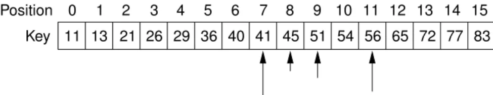
Figure 3.4 illustrates the binary search method. Here is a Java implementation for binary search:
Key
Position 0 2 3 4 5 6 7 8 26 29 36
10 11 12 13 14 15
11 13 21 41 45 51 54
1
56 65 72 77 9
83 40
Figure 3.4 An illustration of binary search on a sorted array of 16 positions.
Consider a search for the position with valueK= 45. Binary search first checks the value at position 7. Because41< K, the desired value cannot appear in any position below 7 in the array. Next, binary search checks the value at position 11.
Because56 > K, the desired value (if it exists) must be between positions 7 and 11. Position 9 is checked next. Again, its value is too great. The final search is at position 8, which contains the desired value. Thus, functionbinaryreturns position 8. Alternatively, ifK were 44, then the same series of record accesses would be made. After checking position 8,binarywould return a value ofn, indicating that the search is unsuccessful.
// Return the position of an element in sorted array "A"
// with value "K". If "K" is not in "A", return A.length.
static int binary(int[] A, int K) { int l = -1;
int r = A.length; // l and r are beyond array bounds while (l+1 != r) { // Stop when l and r meet
int i = (l+r)/2; // Check middle of remaining subarray if (K < A[i]) r = i; // In left half
if (K == A[i]) return i; // Found it if (K > A[i]) l = i; // In right half }
return A.length; // Search value not in A }
To find the cost of this algorithm in the worst case, we can model the running time as a recurrence and then find the closed-form solution. Each recursive call tobinarycuts the size of the array approximately in half, so we can model the worst-case cost as follows, assuming for simplicity thatnis a power of two.
T(n) =T(n/2) + 1forn >1; T(1) = 1.
If we expand the recurrence, we find that we can do so onlylogntimes before we reach the base case, and each expansion adds one to the cost. Thus, the closed- form solution for the recurrence isT(n) = logn.
Functionbinaryis designed to find the (single) occurrence ofK and return its position. A special value is returned if K does not appear in the array. This algorithm can be modified to implement variations such as returning the position of the first occurrence ofK in the array if multiple occurrences are allowed, and returning the position of the greatest value less thanKwhenKis not in the array.
Comparing sequential search to binary search, we see that asngrows, theΘ(n) running time for sequential search in the average and worst cases quickly becomes much greater than theΘ(logn)running time for binary search. Taken in isolation, binary search appears to be much more efficient than sequential search. This is despite the fact that the constant factor for binary search is greater than that for sequential search, because the calculation for the next search position in binary search is more expensive than just incrementing the current position, as sequential search does.
Note however that the running time for sequential search will be roughly the same regardless of whether or not the array values are stored in order. In contrast, binary search requires that the array values be ordered from lowest to highest. De- pending on the context in which binary search is to be used, this requirement for a sorted array could be detrimental to the running time of a complete program, be- cause maintaining the values in sorted order requires to greater cost when inserting new elements into the array. This is an example of a tradeoff between the advan- tage of binary search during search and the disadvantage related to maintaining a sorted array. Only in the context of the complete problem to be solved can we know whether the advantage outweighs the disadvantage.
3.6 Analyzing Problems
You most often use the techniques of “algorithm” analysis to analyze an algorithm, or the instantiation of an algorithm as a program. You can also use these same techniques to analyze the cost of a problem. It should make sense to you to say that the upper bound for a problem cannot be worse than the upper bound for the best algorithm that we know for that problem. But what does it mean to give a lower bound for a problem?
Consider a graph of cost over all inputs of a given sizenfor some algorithm for a given problem. DefineAto be the collection of all algorithms that solve the problem (theoretically, there an infinite number of such algorithms). Now, consider the collection of all the graphs for all of the (infinitely many) algorithms inA. The worst case lower bound is theleastof all thehighestpoints on all the graphs.
It is much easier to show that an algorithm (or program) is inΩ(f(n))than it is to show that a problem is inΩ(f(n)). For a problem to be in Ω(f(n))means thateveryalgorithm that solves the problem is inΩ(f(n)), even algorithms that we have not thought of!
So far all of our examples of algorithm analysis give “obvious” results, with big-Oh always matchingΩ. To understand how big-Oh, Ω, and Θnotations are
properly used to describe our understanding of a problem or an algorithm, it is best to consider an example where you do not already know a lot about the problem.
Let us look ahead to analyzing the problem of sorting to see how this process works. What is the least possible cost for any sorting algorithm in the worst case?
The algorithm must at least look at every element in the input, just to determine that the input is truly sorted. It is also possible that each of thenvalues must be moved to another location in the sorted output. Thus, any sorting algorithm must take at leastcntime. For many problems, this observation that each of theninputs must be looked at leads to an easyΩ(n)lower bound.
In your previous study of computer science, you have probably seen an example of a sorting algorithm whose running time is inO(n2)in the worst case. The simple Bubble Sort and Insertion Sort algorithms typically given as examples in a first year programming course have worst case running times inO(n2). Thus, the problem of sorting can be said to have an upper bound inO(n2). How do we close the gap betweenΩ(n)andO(n2)? Can there be a better sorting algorithm? If you can think of no algorithm whose worst-case growth rate is better thanO(n2), and if you have discovered no analysis technique to show that the least cost for the problem of sorting in the worst case is greater than Ω(n), then you cannot know for sure whether or not there is a better algorithm.
Chapter 7 presents sorting algorithms whose running time is inO(nlogn)for the worst case. This greatly narrows the gap. Witht his new knowledge, we now have a lower bound inΩ(n)and an upper bound inO(nlogn). Should we search for a faster algorithm? Many have tried, without success. Fortunately (or perhaps unfortunately?), Chapter 7 also includes a proof that any sorting algorithm must have running time inΩ(nlogn)in the worst case.2 This proof is one of the most important results in the field of algorithm analysis, and it means that no sorting algorithm can possibly run faster thancnlognfor the worst-case input of sizen. Thus, we can conclude that the problem of sorting isΘ(nlogn)in the worst case, because the upper and lower bounds have met.
Knowing the lower bound for a problem does not give you a good algorithm.
But it does help you to know when to stop looking. If the lower bound for the problem matches the upper bound for the algorithm (within a constant factor), then we know that we can find an algorithm that is better only by a constant factor.
2While it is fortunate to know the truth, it is unfortunate that sorting isΘ(nlogn)rather than Θ(n)!
3.7 Common Misunderstandings
Asymptotic analysis is one of the most intellectually difficult topics that undergrad- uate computer science majors are confronted with. Most people find growth rates and asymptotic analysis confusing and so develop misconceptions about either the concepts or the terminology. It helps to know what the standard points of confusion are, in hopes of avoiding them.
One problem with differentiating the concepts of upper and lower bounds is that, for most algorithms that you will encounter, it is easy to recognize the true growth rate for that algorithm. Given complete knowledge about a cost function, the upper and lower bound for that cost function are always the same. Thus, the distinction between an upper and a lower bound is only worthwhile when you have incomplete knowledge about the thing being measured. If this distinction is still not clear, reread Section 3.6. We useΘ-notation to indicate that there is no meaningful difference between what we know about the growth rates of the upper and lower bound (which is usually the case for simple algorithms).
It is a common mistake to confuse the concepts of upper bound or lower bound on the one hand, and worst case or best case on the other. The best, worst, or average cases each give us a concrete instance that we can apply to an algorithm description to get a cost measure. The upper and lower bounds describe our under- standing of thegrowth ratefor that cost measure. So to define the growth rate for an algorithm or problem, we need to determine what we are measuring (the best, worst, or average case) and also our description for what we know about the growth rate of that cost measure (big-Oh,Ω, orΘ).
The upper bound for an algorithm is not the same as the worst case for that algorithm for a given input of sizen. What is being bounded is not the actual cost (which you can determine for a given value ofn), but rather thegrowth ratefor the cost. There cannot be a growth rate for a single point, such as a particular value of n. The growthrateapplies to thechangein cost as achangein input size occurs.
Likewise, the lower bound is not the same as the best case for a given sizen. Another common misconception is thinking that the best case for an algorithm occurs when the input size is as small as possible, or that the worst case occurs when the input size is as large as possible. What is correct is that best- and worse- case instances exist for each possible size of input. That is, for all inputs of a given size, sayi, one (or more) of the inputs of sizeiis the best and one (or more) of the inputs of sizeiis the worst. Often (but not always!), we can characterize the best input case for an arbitrary size, and we can characterize the worst input case for an arbitrary size. Ideally, we can determine the growth rate for the best, worst, and average cases as the input size grows.
Example 3.14 What is the growth rate of the best case for sequential search? For any array of sizen, the best case occurs when the value we are looking for appears in the first position of the array. This is true regard- less of the size of the array. Thus, the best case (for arbitrary sizen) occurs when the desired value is in the first ofnpositions, and its cost is 1. It is notcorrect to say that the best case occurs whenn= 1.
Example 3.15 Imagine drawing a graph to show the cost of finding the maximum value among n values, as ngrows. That is, the x axis would ben, and they value would be the cost. Of course, this is a diagonal line going up to the right, asnincreases (you might want to sketch this graph for yourself before reading further).
Now, imagine the graph showing the cost foreachinstance of the prob- lem of finding the maximum value among (say) 20 elements in an array.
The first position along thexaxis of the graph might correspond to having the maximum element in the first position of the array. The second position along thexaxis of the graph might correspond to having the maximum el- ement in the second position of the array, and so on. Of course, the cost is always 20. Therefore, the graph would be a horizontal line with value 20.
You should sketch this graph for yourself.
Now, let’s switch to the problem of doing a sequential search for a given value in an array. Think about the graph showing all the problem instances of size 20. The first problem instance might be when the value we search for is in the first position of the array. This has cost 1. The second problem instance might be when the value we search for is in the second position of the array. This has cost 2. And so on. If we arrange the problem instances of size 20 from least expensive on the left to most expensive on the right, we see that the graph forms a diagonal line from lower left (with value 0) to upper right (with value 20). Sketch this graph for yourself.
Finally, lets consider the cost for performing sequential search as the size of the arrayngets bigger. What will this graph look like? Unfortu- nately, there’s not one simple answer, as there was for finding the maximum value. The shape of this graph depends on whether we are considering the best case cost (that would be a horizontal line with value 1), the worst case cost (that would be a diagonal line with value iat positioni along thex axis), or the average cost (that would be a a diagonal line with valuei/2at
positionialong thexaxis). This is why we must always say that function f(n)is inO(g(n))in the best, average, or worst case! If we leave off which class of inputs we are discussing, we cannot know which cost measure we are referring to for most algorithms.
3.8 Multiple Parameters
Sometimes the proper analysis for an algorithm requires multiple parameters to de- scribe the cost. To illustrate the concept, consider an algorithm to compute the rank ordering for counts of all pixel values in a picture. Pictures are often represented by a two-dimensional array, and a pixel is one cell in the array. The value of a pixel is either the code value for the color, or a value for the intensity of the picture at that pixel. Assume that each pixel can take any integer value in the range 0 toC−1. The problem is to find the number of pixels of each color value and then sort the color values with respect to the number of times each value appears in the picture.
Assume that the picture is a rectangle withP pixels. A pseudocode algorithm to solve the problem follows.
for (i=0; i<C; i++) // Initialize count count[i] = 0;
for (i=0; i<P; i++) // Look at all of the pixels count[value(i)]++; // Increment a pixel value count sort(count); // Sort pixel value counts
In this example,countis an array of sizeCthat stores the number of pixels for each color value. Functionvalue(i)returns the color value for pixeli.
The time for the firstforloop (which initializescount) is based on the num- ber of colors,C. The time for the second loop (which determines the number of pixels with each color) isΘ(P). The time for the final line, the call tosort, de- pends on the cost of the sorting algorithm used. From the discussion of Section 3.6, we can assume that the sorting algorithm has costΘ(PlogP)ifPitems are sorted, thus yieldingΘ(PlogP)as the total algorithm cost.
Is this a good representation for the cost of this algorithm? What is actu- ally being sorted? It is not the pixels, but rather the colors. What ifC is much smaller than P? Then the estimate of Θ(PlogP) is pessimistic, because much fewer thanPitems are being sorted. Instead, we should useP as our analysis vari- able for steps that look at each pixel, andC as our analysis variable for steps that look at colors. Then we getΘ(C) for the initialization loop, Θ(P)for the pixel count loop, andΘ(ClogC) for the sorting operation. This yields a total cost of Θ(P+ClogC).