Prediction of pre-breakdown V –I characteristics of an electrostatic precipitator using a combined
boundary element-finite difference approach
B.S. Rajanikanth*, N. Thirumaran
Department of High Voltage Engineering, Indian Institute of Science, Bangalore-560012, India Accepted 1 February 2002
Abstract
A new approach is proposed for the simulation of electrical conditions in a DC energized wire- duct electrostatic precipitator under dust free conditions. Voltage – current characteristics under clean air conditions are considered as a reference in analyzing the performance of a precipitator. This paper gives the simultaneous solution for the governing Poisson’s and current continuity equations using a combined Boundary Element and Finite Difference Method over a one-quarter section of the precipitator. The solution of the domain integral, which represents the effect of space charges in the Poisson’s equation, is also simplified using a numerical technique. The significant features of this paper are, reduced problem domain and hence less memory space and cost, less number of iterations and closer agreement of voltage – current characteristics with published experimental data when compared to other methods. The results are validated against the data obtained from experiments conducted by authors on a laboratory scale precipitator at Bharat Heavy Electricals, Ranipet, India.
The distribution of electric field and current density along the plate have also been presented and discussed in this paper.D2002 Elsevier Science B.V. All rights reserved.
Keywords:Voltage – current characteristics; Precipitator; Boundary element method; Poisson’s equation
1. Introduction
Wire-duct electrostatic precipitators are most commercially used for the removal of solid particulate from combustion flue gases of industries, thereby preventing the emission of toxic particulate into the atmosphere.
0378-3820/02/$ - see front matterD2002 Elsevier Science B.V. All rights reserved.
PII: S 0 3 7 8 - 3 8 2 0 ( 0 2 ) 0 0 0 2 4 - 3
* Corresponding author. Tel.: +91-80-309 2373; fax: +91-80-360 0085/0683.
E-mail address:[email protected] (B.S. Rajanikanth).
www.elsevier.com/locate/fuproc
The performance of an electrostatic precipitator (ESP) can be determined by the voltage – current (V–I) characteristics [1]. TheV–Icurves under clean air conditions help in diagnosing the electrical problems that occur under various load conditions in an existing precipitator. Also, they play an important role in predicting the performance when the ESP is in the design stage for various mechanical input data such as wire radius, wire- to-wire spacing, wire-to-plate spacing, etc. The electrostatic field in the inter-electrode region is governed by Poisson’s and current continuity equations. Several numerical techniques [2 – 8] are being used today, either individually or in combination, for predicting the DCV–Icharacteristics. However, researchers still aim towards improving and refining the existing techniques and minimizing the assumptions made earlier. This will lead to the development of techniques, which give maximum realistic solutions with improved accuracy and faster convergence. Some of the existing numerical techniques related to Finite Difference Method (FDM) and Boundary Element Method (BEM) are reviewed here.
McDonald et al. [2] used FDM, a simple numerical technique, to solve the governing equations. FDM was used to solve both Poisson’s and current continuity equations simultaneously with suitable boundary conditions. The electrical conditions, predicted under dust-free conditions, give a reasonable agreement with experimental data. Electric field strength and space charge densities are calculated as functions of position. However, this method is less accurate and takes more number of iterations when compared to other methods.
Kallio and Stock [3] predicted the electrical conditions in ESPs using a combined Finite Element – Finite Difference method (FE-FD method). While the space charge density was computed using backward difference scheme as was done in Ref. [2], the Poisson’s equation was solved using finite element method with quadratic interpolation. A good agreement was obtained with analytic solution and experimental measurements. Also, this method shows better accuracy and faster computation than the pure FD approach of McDonald et al. [2], and the total number of iterations required by FE-FDM was much less than that required for pure FDM. But, this method uses two different meshes to solve the current continuity and Poisson’s equations. A regular rectangular FD grid, as was used in McDonald’s paper, is used to find out the space charge, whereas the Poisson’s equation is solved using a separate finite element mesh. Further, since the FE nodes are different from the FD nodes, space charges at FE nodes are interpolated from FD point values using a bilinear approximation over each grid rectangle. This makes the computation procedure complicated.
Adamiak [6] simulated the electrical conditions using a combined Boundary Element Method and Method of Characteristics (BEM-MOC). The electric potential was computed using BEM while the charge distribution was found out using MOC. Des- pite its considerable efficiency and speed, this method has a drawback that a full wire section was used to solve the problem against the one-quarter section given by McDonald et al. [2]. This consumes more memory and time. Also, this method uses analytical method to solve the double integral, which represents the charge density in the Poisson’s equation.
In this paper, a novel numerical approach has been proposed using a combined Boundary Element – Finite Difference (BE-FD) method for the solution of governing
equations. This BE-FD combination is being used for the first time in predicting ESP’sV–
Icharacteristics. The combined BE-FD approach is better than either FDM or BE-MOC techniques taken alone, by way of faster convergence and reduced problem domain size (whole section in BE-MOC [6] method, and only a quarter section in the present BE-FD method). The symmetry of the wire – plate geometry facilitates the reduction of the problem domain into a quarter section and the solution can be had for all similar rectangles in the duct. The results were validated with experimental data of Lawless and Sparks [8] and Penney and Matick [9] and other numerically predicted results available in literature. Also, the results have been validated against the data obtained from the experiments, conducted by authors, on a laboratory scale ESP at Bharat Heavy Electricals (BHEL), Ranipet, India [10].
2. Mathematical model
The following general assumptions are made for the mathematical analysis: (i) DC voltage is applied to the wire, (ii) there is no dust in the inter-electrode region, (iii) collection electrodes are clean, (iv) discharge electrode is a round and smooth wire, (v) precipitator works under NTP, and (vi) the mobility of charge carriers is assumed to be uniform and an effective mobility is considered throughout the inter-electrode space.
The mathematical analysis is performed in two-dimensional Cartesian coordinates by solving simultaneously the Poisson’s and current continuity equations, which are given by Eqs. (1) and (2) below, respectively.
j2V ¼ q
e0 ð1Þ
jJ¼0 ð2Þ
Where Vis the applied voltage (kV), q is the space charge density (Coul/m3), e0is the permittivity of air (A s/V m) andJ is the current density (A/m2).
The proposed method is described below in two steps. First, the solution of one of the governing equations, the current continuity equation, by FDM [11 – 13] is explained. The problem domain is similar to that used by McDonald et al. [2]. Then the BEM approach for solving the second governing equation, the Poisson’s equation, is presented finally ending with the complete solution methodology.
2.1. Solution of current continuity equation using FDM
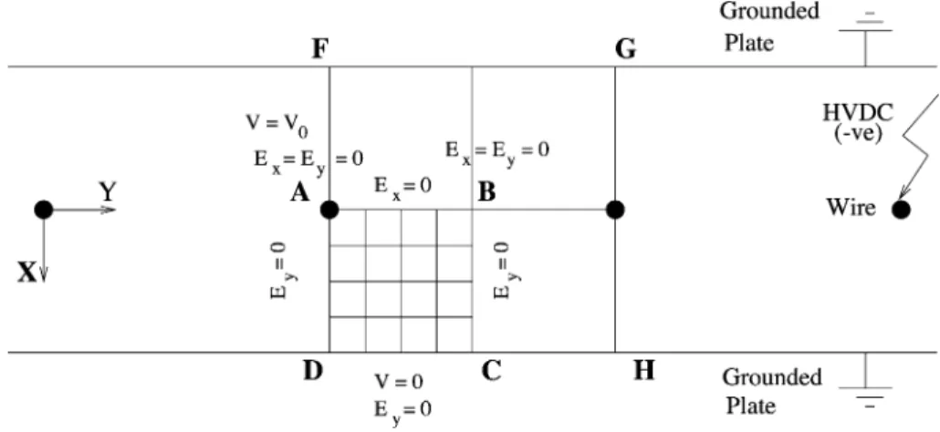
The solution for the current continuity equation using FDM is obtained for the problem domain shown in Fig. 1. The following boundary conditions are applicable here [2]:
(a) ExandEyare zero at points A and B (electric field inxandycoordinates) (b) Ex=DV/Dx= 0 along line AB
(c) Ey=DV/Dy= 0 along lines BC, CD and DA (d) At point A (wire),V=V0and
q¼q0¼ 2JpSy=pa
3:1106f½dþ0:0308ðd=aÞ1=2
Wherefis the roughness factor of the wire (f= 1 for polished wires),dis the air density factor at NTP [2,3],Jpis the average plate current density (A/m2),Syis the half wire-to- wire spacing (m) andais the radius of the wire
(e) V= 0 along line CD
(f) J=qbExon the plate, wherebis the mobility of charge carriers, particularly, that of ions since in a DC-energized ESP majority of the charge carriers in the interelectrode region are unipolar ions.
The continuity (Eq. (2)), expanded using vector algebra, is given by [2],
qbðjEÞ þbðEjqÞ þqðEjbÞ ¼0 ð3Þ Since the mobility of charge carriers is assumed to be constant [1], the third term in Eq. (3) becomes zero. Rewriting the same, one gets
b
e0 q2þ Dq
DxExþDq DyEy
b¼0 ð4Þ
From Eq. (4),qat any point in the grid can be obtained [2].
Fig. 1. Problem domain in a duct-type ESP for solving the current continuity equation.
2.2. Solution for Poisson’s equation using BEM
It should be noted here that, unlike the Adamiak’s BE-MOC method where a full section of ESP is used for modeling, in this paper the authors have shown that only a quarter section of ESP is sufficient enough to be modeled using BE-FD approach.
Referring to Fig. 2, the boundary conditions for solving the Poisson’s equation using BEM are as follows:
(i) At point A (wire lies on point A),V=V0and VV=DV/Dn is unknown (ii) Along line AB,VV= 0 (except at point A) andVis unknown
(iii) Along B1C1,VV= 0 andVis unknown (iv) Along CD,V= 0 andVVis unknown
(v) Along D1A1,VV= 0 andVis unknown.
Referring to Fig. 2, the corners A, B, C and D are split, as each corner has two normal derivatives depending on the side under consideration. Either the potential or its normal derivative has to be known at each point. Since both should not be known at the same point, the potential is given preference and considered as the known quantity while the
Fig. 2. Boundary conditions and split corners.
normal derivative is taken as unknown wherever both quantities are known. For instance, although both voltage Vand normal derivative VV(given by Peek’s formula [14]) are known at point A (which denotes the wire),VVis assumed as an unknown quantity while V=V0is taken as a known one. Further, there are two components of normal derivatives at each corner as shown in Fig. 2. After splitting, points C and D have extra corner points C1
and D1, respectively. According to the boundary condition along line AD, normal derivativeVV(Eyin this case) is zero, whereas according to the boundary condition along line CD, normal derivativeVV(Ex) is an unknown, which has to be found out. If the corner is not split, there will be a problem in selecting the component. Now these two boundary conditions are satisfied after splitting the corner.
2.2.1. Evaluation of potentials at the boundary points
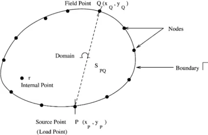
Unlike the domain methods, like FDM and FEM, BEM [15 – 19] is a boundary method, which discretizes only the boundary of the problem geometry. Also, the unknown shape functions can be easily handled as is done in FEM. In BEM, boundary potentials and the normal derivatives are obtained first for the given boundary conditions. Once these values are found out, the interior potentials can be calculated easily with respect to the boundary values. The potentialVat any point P on the boundary can be obtained from the integral equation [15 – 17] as,
CPVP¼ Z
CQ
GP,Q
DVQ
Dn dC Z
CQ
VQDGP,Q
Dn dCþ 1 e0
Z Z
X
qrGP,rdX ð5Þ
and
GP,Q¼ 1 2pln 1
SP,Q
, P,QaCand raX ð6Þ
where CP is a constant and will be explained later; GPQ is the fundamental solution.
Referring to Fig. 3,SPQ¼
ffiffiffiffiffiffiffiffiffiffiffiffiffiffiffiffiffiffiffiffiffiffiffiffiffiffiffiffiffiffiffiffiffiffiffiffiffiffiffiffiffiffiffiffiffiffiffiffi ðxPxQÞ2þ ðyPyQÞ2 q
(distance between the source point P(xP,yP) and field pointQ(xQ,yQ) ),Xis the problem domain,Cis the boundary ofX,Dn is a normal derivative. The subscripts in uppercase letters denote that the points (source or field point) lie on the boundaryC of the problem domain, whereas the lowercase letter subscripts denote that the points lie inside the domainX.
Eq. (5) is the equivalent of Poisson’s equation and can be rewritten as, CPVPþ
Z
CQ
VQ
DGP,Q
Dn dC¼ Z
CQ
DVQ
Dn GP,QdCþ 1 e0
Z Z
X
qrGP,rdX ð7Þ
or
CPVPþ Z
CQ
VGVdC¼ Z
CQ
VVGdCþDP ð8Þ
where,V=VQ,VV=DV/Dn,G=GP,Q,GV=DG/Dn, andDP¼e1
0
Z Z
X
qrGP,rdX(DPrepre- sents the influence of space charge densities on the electrostatic field).
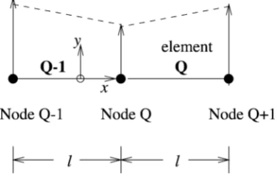
In two-dimensional problems, the boundary of the problem domain is divided into n line segments or elements. Since the variations ofVand VVare assumed to be linear, the boundary is discretized using linear elements (Fig. 4) that have the nodal points at the intersection between two elements, in other words, at the end of each element. Having discretized the rectangular boundary into linear elements, Eq. (8) can be written as,
CPVPþXN
Q¼1
Z
CQ
VGVdC¼XN
Q¼1
Z
CQ
VVGdCþDP ð9Þ
Let us consider an arbitrary segment as shown in Fig. 4. The values ofVandVVat any point of the element can be defined in terms of their nodal values and the linear interpolation functions/1and /2[15,17] as,
VðnÞ ¼/1V1þ/2V2¼ ½/1,/2 V1
V2 2 4
3
5 ð10Þ
VVðnÞ ¼/1V1Vþ/2V2V¼ ½/1,/2 V1V V2V 2 4
3
5 ð11Þ
where, /1¼1
2ð1nÞ ð12Þ
/2¼1
2ð1þnÞ ð13Þ
Fig. 3. Schematic of boundaryCand domainXwith load point (P), field point (Q) and internal point (r).
andn is a dimensionless coordinate and is given by,
n¼x=ðl=2Þ ¼2x=l ð14Þ
wherexis the coordinate point ofnandlis the length of an element. Substituting Eq. (10) forVon the left-hand side of Eq. (9) we get,
Z
CQ
VGVdC¼ Z
CQ
½/1,/2 GVdC V1
V2
2 4
3
5¼ ½aQ1,aQ2
V1
V2
2 4
3
5 ð15Þ
where, aQ1 ¼
Z
CQ
/1GVdC¼ Z
CQ
1
2ð1nÞGVdC, aQ2¼ Z
CQ1
/2GVdC
¼ Z
CQ1
1
2ð1þnÞGVdC ð16Þ
Since nodeQis common to both Qth and (Q1)th elements as shown in Fig. 4, each term is split into two components. The integral on the right-hand side of Eq. (9) becomes,
Z
CQ
VVGdC¼ Z
CQ
½/1,/2 Gd C V1V V2V 2 4
3
5¼ ½bQ1,bQ2 V1V V2V 2 4
3
5 ð17Þ
where,
Fig. 4. Linear element.
bQ1¼ Z
CQ
/1GdC¼ Z
CQ
1
2ð1nÞGdC, bQ2¼ Z
CQ1
/2GdC
¼ Z
CQ1
1
2ð1þnÞGdC ð18Þ
Substituting Eqs. (15) and (17) for all elementsQin Eq. (9), we get the following equation for nodePas:
CPVPþ ½AˆP1,AˆP2, . . . ,AˆPN V1
V2
] VN
2 66 66 66 66 4
3 77 77 77 77 5
¼ ½BP1,BP2, . . . ,BPN
V1V V2V ] VNV 2 66 66 66 66 4
3 77 77 77 77 5
þDP ð19Þ
whereAˆPQ(Q= 1,2,. . .n) terms representaQ1term of elementQplusaQ2term of element Q1 (Eq. (16)), i.e.
Z
CQ
VGVdC¼ Z
CQ
1
2ð1nÞGVdCV1
xA1
þ Z
CQ1
1
2ð1þnÞGVdCV2
xA2
ð20Þ
Similarly,BPQ(Q= 1,2,. . .n) terms representbQ1term of elementQplus bQ2term of elementQ1 (Eq. (18)), i.e.
Z
CQ
VVGdC¼ Z
CQ
1
2ð1nÞGdCV1V xB1
þ Z
CQ1
1
2ð1þnÞGdCV2V xB2
ð21Þ
Therefore, Eq. (19) represents the assembled equation for nodeQ. It can be simplified as,
CPVPþXN
Q¼1
AˆPQVQ¼XN
Q¼1
BPQVQVþDP ð22Þ
or
CPVPþXN
Q¼1
AˆV ¼XN
Q¼1
BVVþDP ð23Þ
whereAˆ¼ Z
CQ
GVdCand B¼ Z
CQ
GdCor XN
Q¼1
AV ¼XN
Q¼1
BVVþDP ð24Þ
where
APQ=AˆPQwhenPpQ APQ=AˆPQ+CPwhenP=Q
The whole set of equations forn number of nodes can be written in matrix form as,
AV¼BVVþD ð25Þ
Eq. (5) or (9) is applicable to any nodal point on the boundary of the problem domain.
The space charge density in the last term is a known quantity, which is obtained using FDM. Since either the potential or its normal derivative is known at each point, a set of algebraic equations is formed to find out the unknown values. In Eq. (25),Dis an n
1 vector consisting of space charge densities,B is an nn coefficient matrix of normal derivatives of potentials andAis annncoefficient matrix of potentials.VandVVare vectors of sizen1.2.2.2. Numerical integration
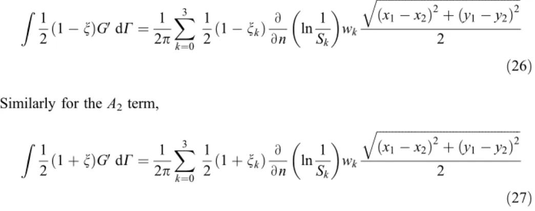
The elements of coefficient matricesAand Bare calculated numerically by using a four-point Gauss quadrature rule [15,17,18,20,21]. The termA1of Eq. (20) is integrated numerically as,
Z 1
2ð1nÞGVdC¼ 1 2p
X3
k¼0
1
2ð1nkÞ D Dn ln 1
Sk
wk
ffiffiffiffiffiffiffiffiffiffiffiffiffiffiffiffiffiffiffiffiffiffiffiffiffiffiffiffiffiffiffiffiffiffiffiffiffiffiffiffiffiffiffiffiffi ðx1x2Þ2þ ðy1y2Þ2 q
2
ð26Þ
Similarly for theA2term, Z 1
2ð1þnÞGVdC¼ 1 2p
X3
k¼0
1
2ð1þnkÞ D Dn ln 1
Sk
wk
ffiffiffiffiffiffiffiffiffiffiffiffiffiffiffiffiffiffiffiffiffiffiffiffiffiffiffiffiffiffiffiffiffiffiffiffiffiffiffiffiffiffiffiffiffi ðx1x2Þ2þ ðy1y2Þ2 q
2
ð27Þ wherex1, y1,x2and y2are the extreme coordinate points of the nodes,nkis the Gauss integration point,Skis the distance between source point and Gauss integration point (Fig. 5)
Fig. 5. Numerical integration using Gauss’ points.
andwkis the weighting factor. Numerical integrations of the B1 and B2 terms of Eq. (21) are given by,
Z 1
2ð1nÞGdC¼ 1 2p
X3
k¼0
1
2ð1nkÞln 1 Sk wk
ffiffiffiffiffiffiffiffiffiffiffiffiffiffiffiffiffiffiffiffiffiffiffiffiffiffiffiffiffiffiffiffiffiffiffiffiffiffiffiffiffiffiffiffiffi ðx1x2Þ2þ ðy1y2Þ2 q
2 ð28Þ
and Z 1
2ð1þnÞGdC¼ 1 2p
X3
k¼0
1
2ð1þnkÞln 1 Sk wk
ffiffiffiffiffiffiffiffiffiffiffiffiffiffiffiffiffiffiffiffiffiffiffiffiffiffiffiffiffiffiffiffiffiffiffiffiffiffiffiffiffiffiffiffiffi ðx1x2Þ2þ ðy1y2Þ2 q
2 ð29Þ
From Eqs. (26) – (29), the off-diagonal elements of coefficient matricesA and B are calculated. The diagonal elements of matrixAare nothing but the constantsCPplus the singular values ofAˆwhich consist of A1 and A2 terms (Eq. (20)) having the integrandDG/
Dnin integral. Singularity comes into picture when the field point lies on the source point itself. The singular elements in matrixAare neglected due to the following reason.
Let us consider the derivativeDGPQ/Dnwhich causes the problem of singularity.
DGPQ
Dn ¼DGPQ
DSPQ DSPQ
Dn
¼DGPQ
DSPQ DSPQ
Dx Dx Dn
þDSPQ
Dy Dy Dn
ð30Þ whereDx/Dn andDy/Dn are the components of the outward normal inxand ydirections, respectively, and are denoted bynxand ny, i.e.,
nx¼Dx
Dn and ny¼Dy
Dn ð31Þ
and, DSPQ
Dx ¼xPxQ
SPQ ; DSPQ
Dy ¼yPyQ
SPQ ð32Þ
From Eqs. (31) and (32), Eq. (30) is rewritten as, DGPQ
Dn ¼DGPQ DSPQ
xPxQ SPQ
nxþ yPyQ SPQ
ny
¼ 1 2p
D DSPQ
ln 1 SPQ
xPxQ SPQ
nxþ yPyQ SPQ
ny
. . . from Eq:ð6Þ
¼ 1
2pS2PQ½ðxPxQÞnxþ ðyPyQÞny ð33Þ
DGPQ
Dn ¼ 1
2pS2PQRn ð34Þ
where
Rn ¼ ðxPxQÞnxþ ðyPyQÞny¼Rn ð35Þ whereR=(xPxQ)+(yPyQ).
In the case of singularity, R and n are orthogonal [19]. Hence, the scalar product becomes zero, which results in the negligence of singular termsAˆin the diagonal elements.
Since the diagonal elements (B1andB2terms of Eq. (21) ) in matrix B are weakly singular, they can be given by the following expression [15,19]
B1 ¼ l
2ð1:5lnlÞ ð36Þ
B2 ¼ l
2ð0:5lnlÞ ð37Þ
wherel¼
ffiffiffiffiffiffiffiffiffiffiffiffiffiffiffiffiffiffiffiffiffiffiffiffiffiffiffiffiffiffiffiffiffiffiffiffiffiffiffiffiffiffiffiffiffi ðx1x2Þ2þ ðy1y2Þ2 q
Once all the elements of the coefficient matricesAandBof Eq. (25) are computed, all unknown vectors with their corresponding coefficients are shifted to the left-hand side while the known ones are on the other side. Now the final matrix form is written as,
ˆaX¼ˆb ð38Þ
whereXis a column vector of unknown potentialsVand their derivativesVV,aˆandbˆare coefficient matrices. The column vector D representing the space charge densities are added with the elements ofbˆ.
2.2.3. Solution of the double integral
The man-hours required for solving the domain integral (DPin Eq. (8)) can be saved by using numerical techniques such as domain celling method [15,22], Monte Carlo method [22], etc. In the domain celling method, the two-dimensional problem-domain is segmented into a collection of triangular subregions or cells. Even though the method seems to be similar to FEM, there are no shape function approximations to the field variables nor are there unknown ones associated with the nodes at the element vertices.
The internal cells are for numerical integration (Gaussian quadrature) purposes only. This method is capable, in principle, of solving the most complex Poisson problems, but at the price of forcing the analyst to discretize and serially index the domain. Actually, doing this is quite time-consuming and expensive. Further, making a mesh eliminates one of BEM’s primary advantages over the domain-based techniques—i.e. the reduction of the dimen- sionality of the problem.
On the other hand, the Monte Carlo quadrature, a numerical technique for solving the domain integral, considers the integral as a whole instead of a piecewise integration over a series of cells. The domain integralDPis evaluated as,
DP ¼ Z Z
X
qrGP,rdX¼qrGP,r Ad¼XM
r¼1
qrGP,r
M Ad ð39Þ
whereqrGP;rdenotes the mean value of the integrand,Adis the total area of the enclosed domain, and M is the total number of sampling points (grid points in this case). This method has the obvious advantage that it is conceptually quite simple and easy to program. In this paper, the Monte Carlo method is employed for solving the domain integral.
2.2.4. Evaluation of potentials at the internal points
Once the boundary potentials and their normal derivatives are calculated, the potential at any internal pointrcan be obtained from the following expression
CrVr¼ Z
CQ
Gr,Q
DVQ
Dn dC Z
CQ
VQDGr,Q
Dn dCþ 1 e0
Z Z
X
qrGr,QdX ð40Þ where Cr at any point rinside the domain is unity. This equation is similar to Eq. (5) except that the load point now is internal pointr.
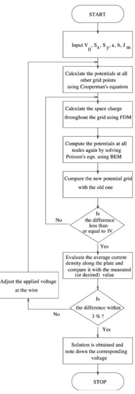
The algorithm for the combined FD-BE approach is as follows.
(a) Assume an initial value of voltage at the wire and calculate the potentials at all other points using Cooperman’s equation [2].
(b) Compute the charge density (q) at all nodes using FDM.
(c) Find out the potentials at all grid points again by solving the Poisson’s equation using BEM.
(d) Repeat steps (b) and (c) until the difference between the new value of Vin the potential grid and its previous value is negligibly small, preferably, say 1 V.
(e) Compute average current density at the plate using
Jp ¼1 n
Xn
j¼1
qjbExj ð41Þ
wheren is the number of equi-spaced grid points along the plate.
(f) Compare the computed and desired average current densities (Jp and Jm) for convergence. If the former is not within 3% of the latter, then adjust the assumed value of voltage and repeat the procedure from step (a) until the convergence is obtained. The flow chart of the computational process is shown in Fig. 6.
2.3. Numerical data
Calculation of space charge density at the wire is essential as it is given as one of the boundary conditions. Approximating the ionized sheath surrounding the wire as cylin- drical,qccan be expressed in terms of the average current density Jpas [2],
qc¼ 2SyJp pbEiri
ð42Þ whereSy= half wire-to-wire spacing (m),Jp= average current density along the plate (A/
m2),b= effective mobility of charge carriers (m2/V s) andri= radius of the ionized sheath (m).
Fig. 6. Flow chart for the combined BE-FD model.
It is assumed that there is no space charge distortion of the field within the ionization region. Therefore,Eirican be approximately taken asEcr, whereEcris the corona onset field given by Peek’s formula [14] as:
Ec¼3:1106fðdþ0:0308 ffiffiffiffiffiffiffi pd=r
Þ ð43Þ
whereris the radius of the wire,fis the roughness factor of the wire (f= 1 for polished wires) andd is the air density factor at NTP.
3. Results and discussions
The previous section described how the solution of Poisson’s and current continuity equations are obtained simultaneously. This is implemented by means of a computer program, which gives the potentials, space charge densities and electric field at all points of the rectangular grid (Fig. 1) of size 15
15. From this, the average current density is calculated along the plate. Assumed initial voltage at the wire, wire radius, half wire-to- wire spacing, wire-to-plate spacing, measured (or assumed) current density at the plate, effective mobility of the charge carriers, air density factor at NTP and roughness factor of the wire are the required input data to be given to the program. The initial estimation of potentials is used to find out the space charge densities throughout the grid using FDM.The calculated charge densities are used in the Poisson’s equation which is then solved by BEM.
3.1. Validation of the model against published experimental data and analytical solutions Figs. 7 – 9 show theV–Icharacteristics for various input data available in the literature.
The predicted result is compared with the Penney and Matick’s [9] experimental data which is usually considered as a reference by researchers. Fig. 7(a) shows the comparison of these two results. Here the calculated current density is less than 2% of the measured value except for the second value (2.2596
104 A/m2), which gives an error of 4%.This error can be reduced by properly selecting the mobility of the charge carriers. This shows that the accuracy also depends on the assumed mobility of the charge carriers. A comparison between the Penney and Matick’s [9] experimental results and theoretical studies is shown in Fig. 7(b). It should be noted here that the proposed BE-FD technique gives much better results than FEM [3] and FDM [2]. The calculated current density lies within 2% of the measured value.
Fig. 8(a) shows the comparison between the experimental results of Lawless and Sparks [8] and predicted results. Here the difference between calculated and measured current densities is less than 2% and the corresponding difference in voltages also lies within 2%.
The mobility used in the calculation was 1.82
104m2/V s as was done by Lawless and Sparks [8]. Fig. 8(b) shows the characteristic curves of Cooperman’s [23] experimental data and predictions made by numerical techniques. Also, the results of Cooperman [24]Fig. 7. Validation of predictedV–Icurves with published experimental data [3,9].
are shown in the same figure. The difference between the measured and the calculated current density is less than 2%. Fig. 9 shows a comparison between the proposed method and analytical methods of Cooperman [23], Sekar and Stomberg [25] and McLean [26]. It
Fig. 8. Validation of predictedV–Icurves with published experimental data [8,23,24].
is observed from the figure that the error between the results of proposed and analytical methods is less than 4%.
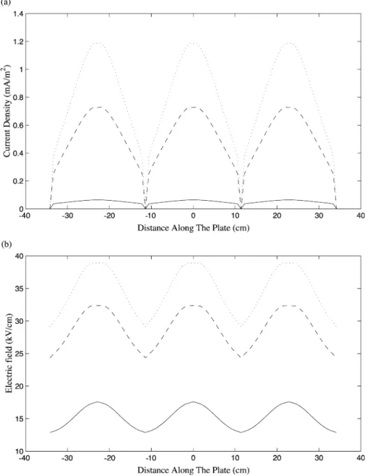
The solid curves in Fig. 10(a) and (b) show the current density and electric field distributions along the plate for a corresponding applied voltage below corona onset. The distribution of current is almost uniform along the plate when the current is below corona onset, whereas the corresponding field shows a periodic distribution with maxima directly under each wire and minima midway between wires. For higher values of current densities, the magnitude of the field increases over the plate. Also, the peak value increases as the current is increased. Current is also maximum directly under the wire and starts decreasing towards the midway between wires for higher values of current densities (dashed and dotted curves of Fig. 10a).
The potential, electric field and charge density distributions along the linear segment extending directly (maximum stress line AD of Fig. 1) from wire to plate are shown in Fig.
11 for Penney and Matick’s [9] experimental data. The magnitudes of voltage and electric field along the maximum stress line are increased due to the presence of space charge. The dashed line represents the distribution of the above-mentioned parameters in the absence of space charges (Lapalcian field). The other three curves show the same parameters for various applied voltages and current densities (i.e. with space charges). The higher the value of
Fig. 9. Validation of predictedV–Icurves with published analytical results [26].
Fig. 10. (a) Current and (b) electric field distribution along the plate for various current densities. Input data: wire radiusa= 1.59 mm; wire – plate spacingSx= 11.4 cm; half wire – wire spacingSy= 11.4 cm; mobilityb= 1.82104 m2/V s; roughness factorf= 1.0; air density factord= 1.0 [8]. Solid line ( __ )Jm= 0.05 mA/m2; dashed line (- - -) Jm= 0.5 mA/m2; dotted line (. . .)Jm= 0.8 mA/m2.
current density, the higher will be the magnitudes of potential, field and charge. Even though there is an increase in the magnitude of the potential and field, there is not much distortion due to the presence of space charge.
Fig. 12(a) – (c) shows the equipotential and field lines for a three-wire section for various current densities. Laplacian field (without space charge) is shown in Fig. 12(a),
Fig. 11. Distribution of (a) potential, (b) field and (c) charge density along the maximum stress line (line AD of Fig. 1) for various current densities. Input data: wire radius = 1.016 mm; wire – plate spacingSx= 11.43 cm; half wire – wire spacingSy= 7.62 cm; mobilityb= 2.0104[9]. Dashed line (- - -)V= 30 kVandJm= 0; solid line ( __ ) V= 38.7 kV andJm= 2.26 mA/m2; dotted line (. . .)V= 43.5 kV andJm= 0.49 mA/m2; dash-dot line (- . -) V= 46.2 kV andJm= 0.69 mA/m2.
Fig. 12. Equipotential and field lines for a three-wire section for various current densities. Input data: wire radius a= 1.59 mm; wire – plate spacingSx= 11.4 cm; half wire – wire spacingSy= 11.4 cm; mobilityb= 1.82104 m2/V s; roughness factorf= 1.0; air density factord= 1.0 [8].
Fig. 13. Potential contours and electric field lines for a quarter section. Input data: wire radiusa= 1.59 mm; wire – plate spacingSx= 11.4 cm; half wire – wire spacingSy= 11.4 cm; mobilityb= 1.82104m2/V s; roughness factor f= 1.0; air density factord= 1.0 [8].
whereas Fig. 12(b) and (c) shows the Poissonian field (with space charge) for 0.5 and 0.8 mA/m2current densities, respectively. It is clear from the figures that the presence of the space charge modifies both the potential and electric field distributions. In particular, the
Fig. 14. Validation of predictedV–Icharacteristics with experimental results from BHEL (a) for three wires and (b) for four wires [10].
Fig. 15. (a) Current and (b) electric field distribution along the plate for various current densities. Input data: wire radius = 0.19 mm; wire – plate spacing Sx= 20 cm; half wire – wire spacing Sy= 7.75 cm; mobilityb= 1.6104m2/ V s; roughness factorf= 1.0; air density factord= 1.0 [10]. Solid line ( __ )Jm= 0.05625 mA/m2; dashed line (- - -) Jm= 0.125 mA/m2; dotted line (. . .)Jm= 0.2125 mA/m2.
equipotential lines become denser in the low field region, which corresponds to an increase of the electric field near the grounded plate. The density of the equipotential lines become more, as the current density increases (Fig. 12a and b). Lawless and Sparks’ [8]
Fig. 16. Distribution of (a) potential, (b) field and (c) charge density along the maximum stress line (line AD of Fig. 1) for various current densities. Input data: wire radius = 0.19 mm; wire – plate spacingSx= 15 cm; half wire – wire spacingSy= 13 cm; mobilityb= 1.6104m2/V s; roughness factorf= 1.0; air density factord= 1.0 [10].
Solid line ( __ )V= 18 kV andJm= 0.06 mA/m2; dashed line (- - -)V= 22 kV andJm= 0.125 mA/m2; dotted line (. . .)V= 26 kV andJm= 0.2125 mA/m2.
experimental data were used as the input here. Fig. 13 shows the corresponding equipotential and field lines for a quarter section of the ESP.
3.2. Validation of the proposed method with experiments conducted at BHEL, India The results from the simulation have also been validated against the data obtained from experiments conducted in a laboratory scale precipitator at Bharat Heavy Electricals (BHEL), Ranipet, India. The corona electrodes were straight and smooth wires of diameter 0.38 mm and were energized by a negative DC supply of rating 100 kV. Wires were placed midway between the parallel plates of area 500
400 mm2. Both plates were grounded through a microammeter. Before the microammeter was connected, the spark-over voltage was determined. The applied voltage was increased slowly and the corresponding voltages and currents were noted down. In order to protect the microammeter, the voltage was applied below 80% of the spark-over voltage. Experiments were done for various wire-to- plate and wire-to-wire spacings. At first, three wires were fixed at an equal wire-to-wire spacing of 15.5 cm. The wire-to-plate spacing was varied as 15, 20 and 25 cm. The experiments were then repeated for a wire-to-wire spacing of 26 cm.Fig. 14 shows the validation ofV–Icharacteristics with the experimental results. The calculation of current density is done for a 15
15 grid. The calculated average current density lies within 4% of the measured current density, but the corresponding difference between calculated and measured voltages is less than or equal to 10%. The V–I characteristics for three and four wires for various wire-to-plate spacings are shown in Fig. 14(a) and (b), respectively.Figs. 15 and 16 plotted for the BHEL experimental data are similar to those shown in the previous sections.
4. Conclusions
In this paper, theV–Icharacteristics of an ESP have been modeled using a combined FD-BE technique. This novel numerical method solves the governing current continuity and Poisson’s equations respectively by FDM and BEM. The combination of these two methods itself is a unique one and is being used for the first time in ESP technology. A 15
15 rectangular grid for the problem domain (quarter section) is used for the entire simulation work as it gives agreeable results. The increase in grid size (2020 or 3030) does not make much difference in obtaining better accuracy. Also, larger grids consume more time and memory.The main and important contribution of this present research work is the reduction of problem domain from a whole section of ESP (as in the previous BE method) to just a quarter section, thus reducing the memory space. Once the solution of governing equations had been obtained for a quarter section, the images of the potentials can be taken throughout the geometry, as it is a symmetric one. Hence, it was enough to restrict the problem-area of interest to a quarter section. Another important feature of this work is that the man-hours required for solving the domain integral by analytical method have been saved by adopting a numerical technique. The inner loop in the
computational process takes three or four iterations while the outer one takes five or six at most.
The proposed method shows good agreement with the published experimental and analytical results. Also, this new approach gives closer agreement with the experimental data when compared with other numerical studies. A maximum of 5% is observed between the predicted results and published data.
From the comparison between the calculated and experimental data obtained from BHEL, it is observed that the difference between the calculated and measured current densities is less than 4% and the corresponding error in voltages is less than 10%. In addition to the analysis of voltage – current characteristics, other electrical conditions such as electric field, current density and charge density have also been discussed in this paper.
References
[1] S. Oglesby Jr., G.B. Nichols, Electrostatic Precipitation, Marcel-Dekker, New York, USA, 1978.
[2] J.R. McDonald, W.B. Smith, H.W. Spencer III, L.E. Sparks, A mathematical model for calculating electrical conditions in wire-duct electrostatic precipitator devices, J. Appl. Phys. 48 (1977) 2231 – 2243.
[3] G.A. Kallio, D.E. Stock, Computation of electrical conditions inside wire-duct electrostatic precipitators using a combined finite-element, finite-difference technique, J. Appl. Phys. 59 (1986) 1799 – 1806.
[4] A.A. Elmoursi, G.S.P. Castle, Modeling of corona characteristics in a wire-duct precipitator using the charge simulation technique, IEEE Trans. IAS 23 (1987) 95 – 102.
[5] S. Cristina, G. Dinelli, M. Feliziani, Numerical computation of corona space charge andV–Icharacteristics in DC electrostatic precipitator, Proc. IEEE Trans. IAS Annu. Meet., California, USA, (1989) 2007 – 2013.
[6] K. Adamiak, Simulation of corona in wire-duct electrostatic precipitator by means of the boundary element method, IEEE IAS Annu. Meet., (1991) 610 – 615.
[7] A.J. Medlin, Electrohydrodynamic modeling of fine particle collection in electrostatic precipitators, PhD Thesis, School of Physics, University of New South Wales, May (1998).
[8] P.A. Lawless, L.E. Sparks, A mathematical model for back corona in wire-duct precipitators, J. Appl. Phys.
51 (1980) 242 – 256.
[9] G.W. Penney, R.E. Matick, Potentials in DC corona fields, Trans. AIEE, Part I 79 (1960) 91 – 99.
[10] N. Thirumaran, A Modified approach to predict voltage – current characteristics of an electrostatic precip- itator, MSc (Engg) Thesis, Department of High Voltage Engineering, Indian Institute of Science, Bangalore, India (2000).
[11] G.D. Smith, Numerical Solution of Partial Differential Equations: Finite Difference Methods, Oxford Univ.
Press, Oxford, 1986.
[12] S.J. Farlow, Partial Differential Equations for Scientists and Engineers, Dover Publications, New York, 1993.
[13] W.F. Ames, Numerical Methods for Partial Differential Equations, Academic Press, New York, 1992.
[14] F.W. Peek Jr., Dielectric Phenomena in High Voltage Engineering, McGraw-Hill, New York, USA, 1929.
[15] C.A. Brebbia, Boundary Element Method for Engineers, Pentech Press, London, 1980.
[16] C.A. Brebbia, J.C.F. Telles, I.C. Wrobel, Boundary Element Techniques, Springer, Berlin, 1984.
[17] C.A. Brebbia, J. Dominguez, Boundary Elements—An Introductory Course, Computational Mechanics Publications, McGraw-Hill, New York, 1988.
[18] F. Paris, J. Canas, Boundary Element Method—Fundamentals and Applications, Oxford Univ. Press, New York, USA, 1997.
[19] F. Hartmann, Introduction to Boundary Elements, Springer, Berlin, 1987.
[20] C.T.H. Baker, The Numerical Treatment of Integral Equations, Clarendon Press, Oxford, 1977.
[21] A.H. Stroud, D. Secrest, Gaussian Quadrature Formulas, Prentice-Hall, New York, USA, 1966.
[22] G.S. Gipson, Progress in the analysis of Poisson type problems by boundary elements, in: C.A. Brebbia (Ed.), Heat Transfer, Fluid Flow and Electrical Applications, Tenth International Conference on BEM,
Boundary Elements X, vol. 2, Computational Mechanics Publications, Springer, Southampton, 1988, pp.
101 – 113.
[23] G. Cooperman, A new voltage – current relation for duct precipitators valid for low and high current densities, IEEE Trans. IAS 17 (1981) 236 – 239.
[24] P. Cooperman, A theory for space charge limited currents with applications to electrostatic precipitation, Trans. AIEE, Part I, (1960) 47 – 50.
[25] S. Sekar, H. Stomberg, On the prediction of current – voltage characteristics for wire-plate electrostatic precipitators, J. Electrost. 10 (1981) 35 – 43.
[26] K.J. McLean, Electrostatic precipitators, IEEE Proc. Part A 135 (1988) 347 – 361.

![Fig. 7. Validation of predicted V –I curves with published experimental data [3,9].](https://thumb-ap.123doks.com/thumbv2/azpdfnet/10624930.0/16.702.86.613.160.864/fig-validation-predicted-v-curves-published-experimental-data.webp)
![Fig. 8. Validation of predicted V –I curves with published experimental data [8,23,24].](https://thumb-ap.123doks.com/thumbv2/azpdfnet/10624930.0/17.702.92.617.75.803/fig-validation-predicted-v-curves-published-experimental-data.webp)
![Fig. 9. Validation of predicted V –I curves with published analytical results [26].](https://thumb-ap.123doks.com/thumbv2/azpdfnet/10624930.0/18.702.84.607.88.538/fig-validation-predicted-v-curves-published-analytical-results.webp)