Full Terms & Conditions of access and use can be found at
http://www.tandfonline.com/action/journalInformation?journalCode=ubes20
Download by: [Universitas Maritim Raja Ali Haji] Date: 12 January 2016, At: 23:44
Journal of Business & Economic Statistics
ISSN: 0735-0015 (Print) 1537-2707 (Online) Journal homepage: http://www.tandfonline.com/loi/ubes20
Dynamic Forecasts of Qualitative Variables
Michael Dueker
To cite this article: Michael Dueker (2005) Dynamic Forecasts of Qualitative Variables, Journal of Business & Economic Statistics, 23:1, 96-104, DOI: 10.1198/073500104000000613
To link to this article: http://dx.doi.org/10.1198/073500104000000613
View supplementary material
Published online: 01 Jan 2012.
Submit your article to this journal
Article views: 164
View related articles
Dynamic Forecasts of Qualitative Variables:
A Qual VAR Model of U.S. Recessions
Michael D
UEKERFederal Reserve Bank of St. Louis, St. Louis, MO 63166 (mdueker@stls.frb.org)
This article presents a new Qual VAR model for incorporating information from qualitative and/or dis-crete variables in vector autoregressions. With a Qual VAR, it is possible to create dynamic forecasts of the qualitative variable using standard VAR projections. Previous forecasting methods for qualitative vari-ables, in contrast, produce only static forecasts. I apply the Qual VAR to forecasting the 2001 business recession out of sample and to analyzing the Romer and Romer narrative measure of monetary policy con-tractions as an endogenous variable in a VAR. Out of sample, the model predicts the timing of the 2001 recession quite well relative to the recession probabilities put forth at the time by professional forecasters. Qual VARs—which include information about the qualitative variable—can also enhance the quality of density forecasts of the other variables in the system.
KEY WORDS: Dummy endogenous variable; Dynamic probit; Recession forecasting.
1. INTRODUCTION
The vector autoregression (VAR) is a standard tool for fore-casting macroeconomic time series, in large part because VARs produce dynamic forecasts that are consistent across equations and forecast horizons. Forecasts are dynamic if the system’s (k+1)-period-ahead forecasts are functions of the system’s k-period-ahead forecasts. Until now, however, the VAR ap-proach has not been applied to forecasting qualitative variables, although qualitative variables have been used as exogenous variables in VARs (e.g., Eichenbaum and Evans 1995). Con-sequently, previous methods of forecasting qualitative variables have not produced dynamic forecasts; instead, the norm is to make static forecasts using lagged values of the explanatory variables, where the minimum lag length equals the forecast horizon. Estrella and Mishkin (1998) and Birchenhall, Jessen, Osborn, and Simpson (1999), for example, used a simple probit or logit model to forecast the probability of a business reces-sion. This article, in contrast, introduces methods for producing dynamic forecasts of a qualitative variable within a VAR frame-work. I call this the “Qual VAR.” A useful by-product of the Qual VAR is that dynamic forecasts involving the qualitative variable can improve the density forecasts of other variables in the VAR system relative to forecasts that do not use information from the qualitative variable.
I apply the Qual VAR to forecasting U.S. business reces-sions, a binary indicator variable defined by the National Bu-reau of Economic Research (NBER). As the NBER business cycle dating committee strenuously pointed out, their widely cited business cycle turning points are judgmental and are not a deterministic function of observable data. The NBER approach to defining turning points stands in contrast to the approaches of Zellner, Hong, and Min (1991), Canova and Ciccarelli (2000), and others who forecasted turning points defined to be a de-terministic function of output growth. In a second application, I highlight another advantage of the Qual VAR approach—its ability to treat a qualitative variable as an endogenous variable in a VAR. As an example, I analyze the Romer and Romer (1989) narrative measure of monetary policy contractions. Pre-vious analysis of the effects of Romer and Romer episodes as-sumed that each episode was completely exogenous (Romer and Romer 1989; Eichenbaum and Evans 1995; Christiano,
Eichenbaum, and Evans 1999). Shapiro (1994) questioned the exogeneity assumption by showing that such monetary policy contractions were somewhat predictable based on the macro-economic environment at the time.
The ubiquity of qualitative and/or discrete variables in macroeconomics suggests that a melding of vector autore-gressions—a workhorse empirical tool in macroeconomics— with limited-dependent variable econometrics would be useful. The empirical analysis of binary indicators of business re-cessions is only one example. Macroeconomists also study qualitative variables concerning currency and banking crises (Eichengreen, Rose, and Wyplosz 1995; Kaminsky and Reinhart 1999), monetary policy shifts (Romer and Romer 1989; Eichenbaum and Evans 1995; Christiano et al. 1999; Boschen and Mills 1995), exchange rate interventions (Lewis 1995; Kaminsky and Lewis 1996), and the effects of currency unions (Rose and van Wincoop 2001; Frankel and Rose 2002). In the examples listed earlier, the qualitative variable is assumed to be exogenous. In many of these cases, however, a VAR ap-proach in which all variables are treated as endogenous might be useful. Interest rate policy instruments that move by discrete amounts are also used in VARs—by, for example, Bernanke and Blinder (1992) and Sims (1992)—and the Qual VAR could be applied to discrete changes to the target federal funds rate.
The Qual VAR builds on the single-equation dynamic or-dered probit model of Eichengreen, Watson, and Grossman (1985) and Dueker (1999). The Qual VAR is dynamic be-cause lagged dependent variables appear on the right side. A re-lated model is the multivariate probit from Chib and Greenberg (1998) and Chib (2000). The Chib and Greenberg (1998) ap-proach differs from a Qual VAR model in that the former would address the serial correlation found in time series through autoregressive errors, rather than autoregressive variables. In multivariate macroeconometrics, the distinction between au-toregressive variables and auau-toregressive errors is significant. With autoregressive errors, forecasting would require a supple-mentary model to forecast the covariate variables. In a system
© 2005 American Statistical Association Journal of Business & Economic Statistics January 2005, Vol. 23, No. 1 DOI 10.1198/073500104000000613
96
Dueker: Dynamic Forecasts of Qualitative Variables 97
of autoregressive variables, such as a VAR, model-consistent forecasts of all variables are readily available. Moreover, the multivariate probit is set up to emphasize cross-sectional corre-lations among a set of qualitative variables and the coefficients on exogenous covariates. VARs, in contrast, are better suited to a small system of endogenous variables and a relatively large number of autoregressive lags. For this reason, in this article I extend the dynamic probit model to a VAR setting.
Other related models include the autoregressive conditional hazard (ACH) model of Hamilton and Jorda (2002) and the au-toregressive conditional multinomial (ACM) model of Engle and Russell (1998) and Herrera (2003). In the event that one wants to specify these models with a richer set of explanatory variables than the dependent variable’s own history, an auxil-iary model to forecast the covariates is needed with either the ACH or the ACM models. In a Qual VAR, in contrast, all of the covariates are part of the same VAR system, so no auxiliary model is needed for multistep forecasts.
2. QUAL VAR AND ITS ESTIMATION
Our starting point is the dynamic probit model of Eichengreen et al. (1985), which serves as a time series probit because it in-cludes an autoregressive dependent variable. As in simple pro-bit models, one can assume that a continuous latent variable,y∗, lies behind the binary dependent variable,y∈ {0,1},
yt=0 ify∗t ≤0,
yt=1 ify∗t >0,
y∗t =ρy∗t−1+Xt−1β+ǫt, ǫt∼N(0,1),
(1)
whereXt−1is a set of explanatory variables. The fact that the latent variable,y∗, is an autoregressive variable makes the dy-namic probit suitable as an equation in a VAR system. This article extends the single-equation dynamic probit to a VAR system.
The maximum-likelihood estimation procedure of Eichengreen et al. (1985) requires numerical evaluation of an integral for each observation to obtain the density,h, of the la-tent variable,y∗t, whereφ is the standard normal density and Itis the information available up to timet,
h(y∗t|It)=1/σǫ Ut−1
lt−1
φ(y∗t/σǫ)h(y∗t−1|It)dy∗t−1, (2) where{lt,Ut} = {−∞,0}ifyt=0, or{0,∞}ifyt=1. Because
numerical evaluation of these integrals is time-consuming and approximate, Dueker (1999) demonstrated the relative simplic-ity of estimating the dynamic probit model through Markov chain Monte Carlo (MCMC), an approach also applied by Dueker (2000), Dueker and Wesche (2003), and Chauvet and Potter (2003). MCMC estimation of the dynamic probit extends the work of Albert and Chib (1993), who presented MCMC methods for static probit models. In cases like the dynamic pro-bit, where the joint density ofy∗t andy∗t−1is difficult to evaluate, data augmentation via MCMC offers a tractable method to gen-erate (i.e., augment the observed data with) a sample of draws from the joint distribution of they∗through a sequence of draws from the respective conditional distributions. Data augmenta-tion in the present context allows one to treat augmented values
ofy∗s,s=t, as observed data when evaluating the conditional density ofy∗t. Thus one conditions the density ofy∗t on avalue, instead of adensity, ofy∗t−1, making the problem much simpler than recursive evaluation of the integral in (2). This argument in favor MCMC estimation methods applies, and is even ampli-fied, if the latent variabley∗is in a VAR, as opposed to a single equation. Most important, in a VAR, standard forecasting meth-ods can be applied to predict futurey∗.
2.1 MCMC Sampling for the Qual VAR
A Qual VAR model withkvariables andplags can be written as
consists of macroeconomic data,Xt, plus the latent variable,y∗; (L) is a set ofk×k matrices, from L=0, . . . ,p, with the identity matrix at L=0; µ is a set of intercepts; and ǫ are mean-0 normally distributed disturbances. The covariance ma-trix of the forecast errors is denoted by . The parameters that require conditional distributions for MCMC estimation are—the VAR regression coefficients—the covariance ma-trix,, and the latent variable,y∗.
MCMC is an attractive estimation procedure for the Qual VAR, because deriving the conditional distribution of the la-tent variable is straightforward, given the VAR coefficients; in turn, the conditional distributions of the VAR coefficients sim-ply have the ordinary least squares (OLS) distribution, given values for the latent variable. The key idea behind MCMC esti-mation is that after a sufficient number of iterations, the draws from the respective conditional distributions jointly represent a draw from the joint posterior distribution, which often cannot be evaluated directly (Gelfand and Smith 1990).
MCMC estimation of this model consists of a sequence of draws from the following conditional distributions, where su-perscripts indicate the iteration number:
VAR coefficients∼normal
Covariance matrix∼inverted Wishart f(i+1)
Latent variable∼truncated normal
fy∗(t i+1) (i+1),yj∗(i+1)j<t,y∗(k i)k>t,
{Xt}t=1,...,T,(i+1).
(4)
Conditional on a set of values for y∗ and, the VAR coeffi-cients,, are normally distributed with the mean and variance of the OLS estimator, as implied by an uninformative prior. The covariance matrix is sampled from the inverted Wishart distri-bution, also with an uninformative prior, as discussed by Chib and Greenberg (1996),
As in all probit-type models, the variance of the latent vari-able,y∗, is not identified and must be normalized to an arbitrary value. Consequently, elements of the last row and column of are normalized to preserve correlations when the lower right element is set to unity.
A single period’s value of latent variable, y∗, has a trun-cated normal distribution, wherey∗ is not allowed to be neg-ative during expansions or positive during recessions. Using the conditional mean, µy∗, and variance, σy∗, derived later,
(y∗−µy∗)/σy∗ is in the interval (−∞,0−µy∗/σy∗] during
recessions and(0−µy∗/σy∗,+∞)during expansions. Let the
relevant bounds be denoted by (l,u) and let F be the cumu-lative normal density function. To sample from the truncated normal, we first draw a uniform variable,υ, from the interval
(F(l),F(u)). The truncated normal draw for(y∗−µy∗)/σy∗ is
thenF−1(υ).
In both applications presented later, the MCMC sampler was run for a total of 10,000 iterations. The first 5,000 iterations were discarded to allow the sampler to converge to the poste-rior distribution. Experimentation showed that nearly identical estimates resulted when more than 5,000 initial iterations were discarded. Even though the OLS point estimates of the VAR co-efficients almost never implied a root at or above 1, the draw of randomized VAR coefficients from the OLS distribution some-times did imply an explosive root. These draws were rejected and resampled.
2.2 Conditional Distribution of the Latent Variable
We need to derive the full conditional distribution of y∗t| {Y−t},Xt, where{Y−t}is the full vector time series except for
timetdata. In the application to recession forecasting, the la-tent variabley∗might be called a business cycle index, because its distance from 0 indicates how many standard deviations the economy is from a business cycle turning point. The full condi-tional distribution ofy∗t|{Y−t},Xtcan be expressed as
f(y∗t|{Y−t},Xt)∝f(Yt|{Y−t}). (6) Thus we start by deriving the conditional distribution of
Yt|{Y−t}. Once this conditional distribution has been calcu-lated, results about conditional relationships among multivariate normals can be used to derive f(y∗t|Xt). Because the autore-gressive order is p, the value of Yt will affect the
relation-ship between the observed data and the shocks for the next p+1 periods,
whereis the cross-equation covariance matrix of the errors, which are uncorrelated across time. After collecting all cross-products, we have
Without loss of generality, it can be assumed that the latent vari-able,y∗t, is the last element inYt and partitionCaccordingly,
whereC11is a scalar,
After collecting terms, we have
ˆ
y∗t| ˆXt∼N(−C11−1C′
01Xˆt,C−111). (11)
The conditional mean ofy∗t is the conditional mean ofˆy∗t plus the last element ofC−1D. From this distribution, values ofy∗t are sampled as truncated normals, depending on whether the NBER classifications specify a positive or a negative value ofy∗t.
Exact conditional distributions can be derived in similar fash-ion for the firstpobservations. However, I found that sampling from the exact distributions was very slow numerically, because of the large matrices involved. For these conditional distribu-tions, it was necessary to invert a matrix that isk2p2×k2p2, wherekis the number of variables in the VAR. For this reason, I instead used an accept–reject Metropolis–Hastings (AR–MH) algorithm to sample the firstpvalues of the latent variable at iteration(i+1):
1. For a given value ofj, 1≤j≤p, draw a proposed value of yjpd from the proposal density,fpd(·), which has a mean and variance equal to that of the conditional distribution ofy∗p+1. The proposed values are taken from a truncated normal distribution that respects the recession/expansion categories of the firstptime periods.
2. Given current iteration values for ,,y∗j+1, . . . ,y∗j+p, calculate the densities of the data, Yj, . . . ,Yj+p, at both
the proposed value of yjpd and at the last iteration’s valuey∗(j i).
Dueker: Dynamic Forecasts of Qualitative Variables 99
3. Calculate
Rd=
fpd(yjpd)f(Y|yjpd)
fpd(y∗(i) j )f(Y|y
∗(i)
j )
. (12)
The acceptance probabilities foryjpdare
Rd forRd<1
1 forRd≥1.
Experimentation showed that the results were not much affected by using AR–MH sampling of the first p values of the latent variable, as opposed to Gibbs sampling from the exact condi-tional distributions.
3. A QUAL VAR OF U.S. RECESSIONS
I used quarterly data from 1968:Q1 to 2000:Q3 to estimate a Qual VAR that includes information on U.S. recessions. The data used to estimate the Qual VAR were compiled on Decem-ber 8, 2000, so they do not reflect any revisions to GDP data that occurred after the onset of recession in March 2001. In using the Qual VAR for end-of-sample forecasting, it is assumed to be known that during 2000:Q3 the economy was not in recession. This assumption is not controversial for that particular date, but such an assumption could be problematic at other points in time. For this reason, I focus in this article on out-of-sample forecast results for 12 quarters from 2000:Q4 to 2003:Q3. Fu-ture work can focus on recursive estimation of Qual VARs with real-time datasets, which would have to include real-time data on whether the economy was believed to be in recession.
The recession and expansion classification comes from the NBER. The dates of business cycle turning points are listed in Table 1. The NBER Business Cycle Dating Committee chooses turning point months, which means that one can think that the first half of a turning point month can be considered the last part of the previous recession or expansion, and the second half of the month can be considered part of the next phase of the busi-ness cycle. (This interpretation was provided by Ben Bernanke, former member of the NBER committee.) For this reason, the March 2001 peak, for example, implies that the second quarter of 2001 would be the first quarter of the recession.
The set of macroeconomic variables,X, in the forecasting
VAR include the quarterly growth rate of chain-weighted real GDP, quarterly inflation in the consumer price index, the term spread between yields on 10-year Treasury Bonds and 3-month Treasury Bills, and the effective federal funds rate. Variables such as these have been used to produce forecasts of reces-sions in simple probit models (see, e.g., Estrella and Mishkin 1998). Moreover, each of these variables should reflect sources
Table 1. NBER Business Cycle Turning Points, 1968–2000
Peak Trough
December 1969 (1970:Q1) November 1970 (1970:Q4) November 1973 (1973:Q4) March 1975 (1975:Q1) January 1980 (1980:Q1) July 1980 (1980:Q2) July 1981 (1981:Q3) November 1982 (1982:Q4) July 1990 (1990:Q3) March 1991 (1991:Q1) March 2001 (2001:Q2) November 2001 (2001:Q4)
NOTE: The dates in parentheses show the first and last quarters of the recession.
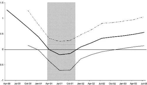
Figure 1. Posterior Mean of Latent Variable With End-of-Sample
Forecasts and 80% Probability Interval for 2000:Q4–2003:Q3
( mean; 80% low; 80% high).
of cyclical strength or weakness. The slope of the yield curve provides a glimpse of whether the bond market anticipates a future drop in procyclical short-term interest rates. The federal funds rate is the monetary policy instrument, and Romer and Romer (1989) claimed that some monetary policy contractions have precipitated recessions.
With the latent variable,y∗, that lies behind the NBER reces-sion/expansion classifications, the VAR has five variables and five lags of each variable. The choice ofp=5 lags was made a priori and reflects the frequent use of a lag length in VARs equal to 1 year plus one lag. Figure 1 shows the posterior mean of the latent business cycle index,y∗, with the NBER recessions shaded. A virtually identical version of Figure 1 was presented to the Board of Directors of the Little Rock Federal Reserve branch on December 15, 2000. The latent variable looks the way one would expect, in that the 1969–1970 and 1990–1991 recessions do not fall as far below 0 as the other recessions. In the out-of-sample period, the latent variable was expected to decline, with point estimates that dip below 0, although the 80% probability interval includes 0 throughout the 12 quarters. The end-of-sample forcasts of the latent variable also predicted a rather tepid recovery from recession in comparison with the slope the latent variable had coming out of previous recessions. Figure 2 highlights the out-of-sample period that starts at the end of 2000. The dynamic forecast of the latent business cycle
Figure 2. End-of-Sample Forecasts of Latent Variable and 80%
Probability Interval Starting in 2000:Q4 ( mean; 80% low;
80% high). The shaded regions are NBER recessions.
variable from the Qual VAR dips below 0 for almost precisely the period that the NBER subsequently defined to be a reces-sion.
The Qual VAR also produces recession probabilities. Dy-namic Qual VAR forecasts of recessions are based on simu-lations of the VAR systemkperiods from the forecast date. The forecasted recession probability is the percentage of iterations where the simulated latent variable was negativekperiods into the future,
ˆ
Yt+k=EYˆ
t+k| ˆYt+k−1+1/2et+k, (13)
whereYˆ denotes a simulated value and eis a vector ofk in-dependent random standard normals. If the simulated value of the latent variable, ˆy∗, which is the last element in Yˆ, is less
than 0 in 30% of the simulation iterations, then the forecasted probability of recession is 30%,
Pr(yt+k=0|It)=
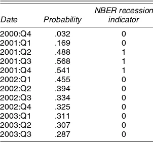
Table 2 presents out-of-sample recession probabilities from the Qual VAR. The rise and fall of the probabilities closely matches the subsequently declared NBER recession period. The fact that the recession probabilities exceed 50% must be viewed in light of previous recession forecasting methods. Birchenhall et al. (1999) investigated ways to translate model-based reces-sion probabilities into yes/no recesreces-sion signals. They consider two key recession probability levels: 50% and 16%, which is their sample average of the percentage of time spent in reces-sions. Dueker (2002) calculated the optimal probability level for 6-month-ahead yes/no recession signals in the case where the loss function puts greater weight on not missing a reces-sion than on falsely predicting a recesreces-sion. The cutoff probabil-ity in that signaling exercise was 28%. Moreover, for horizons greater than two quarters ahead, the optimal cutoff probabil-ity would likely be even lower. Viewed in this context, the Qual VAR forecast five quarters ahead of a recession proba-bility above 50% for 2001:Q3 and 2001:Q4 is a rather strong signal of recession. This is especially true in light of the dif-ficulties that professional forecasters and the leading indicators had in anticipating the 2001 recession. For example, in the Blue Chip forecasters November 2000 survey, the mean probabil-ity that the U.S. economy would enter a recession within the next 12 months was only 23%. In addition, in the September 2001 survey of Blue Chip forecasters, which was completed just before September 11, only 13% believed that the United States had slipped into recession by that date (Source: Blue Chip Economic Indicators, various issues). Stock and Watson (2003) documented the shortcomings of the variables in the Conference Board’s Index of Leading Indicators in signaling the economic downturn in 2001.
The Qual VAR of U.S. recessions also produces useful den-sity forecasts of the macroeconomic variables for 12 quarters out of sample. Here I compare the density forecasts of gross do-mestic product (GDP) growth and consumer price index (CPI) inflation between the Qual VAR and the ordinary VAR that does not include information on the NBER recession classifications.
Table 2. End-of-Sample Forecasts of Recession Probabilities
NOTE: Forecasts are based on data through 2000:Q3.
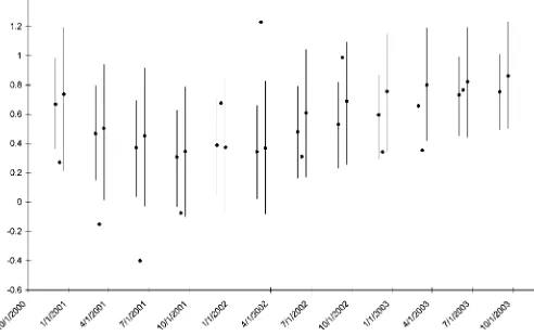
I do not report density forecasts for the federal funds rate, be-cause neither model comes close to predicting the extraordinary drop in the federal funds rate to 1% by June 2003. Both models are estimated by MCMC to simulate 80% probability intervals around the point forecasts. Figures 3 and 4 plot three points for each time period. The left and right points are surrounded by a vertical line indicating the 80% probability interval corre-sponding to the ordinary VAR and Qual VAR. The middle point represents the actual data as of September 8, 2003. As shown in Figure 3, the 80% probability interval for output growth con-tains the actual data in 8 of 11 out-of-sample quarters for the Qual VAR, versus 5 of 11 for the ordinary VAR. Figure 4 shows that the Qual VAR’s 80% probability interval contains the ac-tual data in 7 of 11 forecasts, versus 5 of 11 for ordinary VAR. Thus the Qual VAR probability interval comes closer to cap-turing 80% of the actual observations. It appears that the Qual VAR does better in forecasting how uncertain future outcomes of the state of the business cycle will affect the range of possible outcomes of output growth and inflation.
Another interesting feature of the out-of-sample forecasts is that the Qual VAR predicts a greater than 50% chance of re-cession in 2001, despite the fact that the point forecasts for GDP growth are all above 0. Instead, the point forecasts for
Figure 3. Twelve Quarters of End-of-Sample Forecasts for CPI In-flation. The left vertical line represents the 80% probability interval and point forecast from the ordinary VAR, and the right vertical line has the corresponding information for the Qual VAR. The point between the lines is the actual value.
Dueker: Dynamic Forecasts of Qualitative Variables 101
Figure 4. Twelve Quarters of End-of-Sample Forecasts for GDP Growth. The left vertical line represents the 80% probability interval and point forecast from the ordinary VAR, and the right vertical line has the corresponding information for the Qual VAR. The point between the lines is the actual value.
GDP growth dip to about 0.3% per quarter before rebound-ing. Of course, the Qual VAR does not impose the rule of thumb that a recession consists of at least two negative quar-ters of GDP growth. It is also interesting to note that until the July 2002 annual revision to the GDP, the data showed only one slightly negative quarter, in 2001:Q3. After this substan-tial revision, however, real GDP growth showed three negative quarters, as illustrated in Figure 3. Hence the out-of-sample forecasts would conform much better to the real-time data re-leases than to subsequently revised numbers. The Qual VAR also bolsters the decision of the NBER dating committee to an-nounce a March 2001 business cycle peak on November 26, 2001—a time when the data showed only one slightly nega-tive quarter of GDP growth that could have easily been revised away in the following 2 months. The Qual VAR forecasts sug-gest that a recession not marked by two negative quarters of GDP growth can be consistent with the procedures used to date previous NBER recessions. This is especially true in circum-stances where employment and output growth do not coincide due to strong productivity growth, as was the case throughout much of the period after 2000.
4. A QUAL VAR OF ROMER POLICY CONTRACTIONS
Romer and Romer (1989) carefully studied Federal Reserve documents to identify points in time when monetary policy-makers explicitly decided to initiate disinflation through reces-sion if necessary. These decireces-sion points have become known as “Romer dates” and are used in empirical analysis as a binary qualitative variable. The Qual VAR approach allows qualita-tive variables such as Romer and Romer (1989) monetary pol-icy contractions to be an additional endogenous variable in the system, rather than an exogenous regressor. For Romer dates, I used monthly data, because quarterly data could mix the ini-tial monetary policy decision with its subsequent effects. The data that I include in the VAR are output growth in terms of in-dustrial production (IP), inflation in personal consumption ex-penditure prices (INF), the federal funds rate (FF), and the term spread (TERM) between the yield on 10-year Treasury Bonds
and the federal funds rate. To include a long history of Romer and Romer episodes, I used monthly data from January 1959 to September 1996. The months classified as Romer dates by Choi (1999) and others are March 1959, December 1965, De-cember 1968, April 1974, August 1978, and DeDe-cember 1988. This five-variable Qual VAR includes six monthly lags of the data.
The principal aim here is to examine whether the conclu-sions about the effects of Romer and Romer monetary policy episodes on the economy remain the same when this qualitative variable is treated as endogenous, not exogenous. I am particu-larly interested in whether the impulse responses to a “Romer shock” differ from those reported by Christiano et al. (1999), who treated Romer dates as exogenous. Interstingly, when these authors discussed the proper way to bootstrap confidence in-tervals for impulse responses to Romer shocks, they acknowl-edged that with different shock histories, the Federal Reserve would have chosen different Romer dates. This is tantamount to saying that Romer dates are endogenous, as a Qual VAR would assume from the outset.
The recursive variable ordering that I used to identify impulse responses is
{IP,INF,ROMER,TERM,FF},
whereROMER is the latent variable behind the Romer dates. This ordering purposely puts the interest rates after the Romer latent variable because interest rates can respond within the month in which a Romer policy contraction is initiated. The impulse responses calculated in this way reflect all unantici-pated changes in the latent variable, even those changes that do not cause the latent variable to cross 0. In presenting impulse responses to Romer shocks, however, I normalize the shock to reflect the size of shock that occurred on a typical Romer date, rather than a shock equal to one sample standard devia-tion, which is considerably smaller. In this way, I can compare my results with those of Christiano et al. (1999) regarding, for example, the maximal impact of a Romer date on the level of the federal funds rate.
The impulse responses of all five variables to a Romer shock are shown in Figure 5. The impulse responses of output growth to shocks are not as smooth or persistent as the responses of the level of output would be, but I included variables in station-ary form because the latent Romer variable must be stationstation-ary by definition; monetary policy does not wander arbitrarily far from conditions where a Romer-type policy contraction would occur. Indeed, the response of output growth is choppy for the first 3 months but is significantly negative between 4 and 10 months after a Romer date. Inflation displays the well-known price puzzle, but only between 4 and 6 months. The maximal impact on the federal funds rate from a Romer shock is a little more than 200 basis points and occurs only 3 months after the Romer date. This effect is greater than the estimate of 100 basis points from Christiano et al. (1999). It is perhaps surprising that by treating the Romer date as an endogenous variable, I find a larger maximal impact on the federal funds rate. It turns out that the latent variable often needs a shock of several standard devi-ations to generate the observed Romer dates. The small number
(a) (b)
(c) (d)
(e)
Figure 5. Responses to Romer Shock of (a) Inftation, (b) Output Growth, (c) Term Spread, (d) Federal Funds Rate, and (e) Latent Romer Variable
( lower 10%; top 10%; median).
of Romer dates provides only an imprecise estimate of the aver-age size of the shock to the latent variable at the time of Romer dates. Hence the maximal impact of a Romer date on the federal funds rate is also rather imprecisely estimated. Consequently, the signs and shapes of the Romer impulse responses are esti-mated more reliably than the magnitudes of the responses. As one might expect, the effect of a Romer shock on the latent Romer variable is very transitory, given that Romer dates do not occur in bunches.
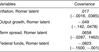
Given that the Qual VAR allows all variables to be contem-poraneously correlated, it is interesting to look at the posterior means of the elements of the covariance matrix that corre-spond with Romer shocks. Table 3 reports the posterior means and 90% probability intervals for these covariances. Because a Romer policy contraction occurs when the latent variable drops below 0, innovations to the latent Romer variable in the direction of policy contraction are associated with a positive
innovation in the federal funds rate and a negative innovation in inflation. The 90% probability intervals for these two covari-ances either do not contain 0 or barely contain it in the case of inflation. Together, these two covariances suggest that Romer
Table 3. Contemporaneous Residual Covariances
Variables Covariance
Inflation, Romer latent .017 (−.0016, .0385) Output growth, Romer latent −.049
(−.142, .0478) Term spread, Romer latent .0658
(−.0287, .1462) Federal funds, Romer latent −.0823
(−.1500,−.001)
NOTE: 90% probability interval is in parentheses.
Dueker: Dynamic Forecasts of Qualitative Variables 103
dates are associated with increases in real interest rates, as one might expect.
5. CONCLUSIONS
This article presents a new Qual VAR model for incorporat-ing information from qualitative variables in VAR models. With a Qual VAR, it is straightforward to create dynamic forecasts of the qualitative variable using standard VAR projections. Previ-ous forecasting methods for qualitative variables, in contrast, provide only static forecasts or require an auxilary model to forecast the covariates. The Qual VAR did quite well in pre-dicting the 2001 recession out of sample. Previous models that attempt to convert recession forecast probabilities into yes/no signals of recession suggest that a 50% recession probability is a strong signal of recession. As an augmented VAR, the Qual VAR—which includes information about the qualitative vari-able in the form of a truncated normal latent varivari-able—can also enhance the quality of density forecasts of other variables in the system, such as output growth, relative to the VAR without the qualitative variable. In the application to business cycle fluctua-tions, the Qual VAR density forecasts widened appropriately to reflect uncertainty about the furture state of the business cycle. Estimation of the Qual VAR takes place through MCMC and requires only draws from normal and uniform distributions. The conditional distributions needed to sample the latent variable that lies behind the qualitative variable are straightforward and easy to implement, with the exception of the firstp values of the latent variable conditional on a VAR(p) process. For the firstpvalues, the sizes of the matrices needed to sample from the conditional distribution are large enough to serve as a bot-tleneck in terms of computation time. For this reason, I sampled the firstpvalues using an AR–MH algorithm that is not com-putationally demanding.
The Qual VAR also addresses the problematic assumption that qualitative variables can be used as exogenous regressors in VARs. In VARs it is common to include qualitative variables to delineate different macroeconomic regimes, such as a gold standard or a fixed exchange rate peg. The assumption that these regime choices are exogenous to the macroeconomic environ-ment is highly questionable. In a Qual VAR, such qualitative variables are simply appended to the VAR system and treated as any other endogenous variable. I have illustrated this endo-geneity feature of the Qual VAR in an application of Romer and Romer (1989) monetary policy contractions. The Qual VAR— provided a recursive ordering assumption frequently used in VARs—implies a set of impulse responses to a shock to the latent variable behind a Romer contraction without assuming that the Romer contraction is an exogenous regressor.
ACKNOWLEDGMENTS
The content of this article is the responsibility of the author and does not reflect an official position of the Federal Reserve Bank of St. Louis or the Federal Reserve System. The author thanks Arnold Zellner, James Hamilton, Ivan Jeliazkov, and two anonymous referees for suggestions and comments.
[Received April 2002. Revised December 2003.]
REFERENCES
Albert, J. H., and Chib, S. (1993), “Bayesian Analysis of Binary and Polychoto-mous Response Data,”Journal of the American Statistical Association, 88, 669–679.
Bernanke, B. S., and Blinder, A. S. (1992), “The Federal Funds Rate and the Channels of Monetary Transmission,”American Economic Review, 82, 901–921.
Birchenhall, C. R., Jessen, H., Osborn, D. R., and Simpson, P. (1999), “Predict-ing U.S. Business-Cycle Regimes,”Journal of Business & Economic Statis-tics, 17, 79–97.
Boschen, J., and Mills, L. (1995), “The Relation Between Narrative and Money Market Indicators of Monetary Policy,”Economic Inquiry, 33, 24–44. Canova, F., and Ciccarelli, M. (2000), “Forecasting and Turning Point
Predic-tions in a Bayesian Panel VAR Model,” Working Paper 443, Universitat Pom-peu Fabra.
Chauvet, M., and Potter, S. (2003), “Predicting Recessions Using the Yield Curve,”Journal of Forecasting, forthcoming.
Chib, S. (2000), “Bayesian Analysis of Correlated Binary Data,” in General-ized Linear Models: A Bayesian Perspective, eds. D. Dey, S. Ghosh, and B. Mallick, New York: Marcel Dekker, pp. 113–131.
Chib, S., and Greenberg, E. (1996), “Markov Chain Monte Carlo Methods in Econometrics,”Econometric Theory, 12, 409–431.
(1998), “Analysis of Multivariate Probit Models,” Biometrika, 85, 347–361.
Choi, W. G. (1999), “Asymmetric Monetary Policy Effects on Interest Rates Across Monetary Policy Stances,”Journal of Money, Credit and Banking, 31, 386–416.
Christiano, L. J., Eichenbaum, M., and Evans, C. L. (1999), “Monetary Pol-icy Shocks: What Have We Learned and to What End?” inHandbook of Macroeconomics 15, eds. J. B. Taylor and M. Woodford, Amsterdam: North-Holland, pp. 65–148.
Dueker, M. (1999), “Conditional Heteroscedasticity in Qualitative Response Models of Time Series: A Gibbs Sampling Approach to the Bank Prime Rate,”Journal of Business & Economic Statistics, 17, 466–472.
(2000), “Are Prime Rate Changes Asymmetric?” Federal Reserve Bank of St. Louis Review, 82, 33–41.
(2002), “Regime-Dependent Recession Forecasts and the 2001 Reces-sion,”Federal Reserve Bank of St. Louis Review, 84, 29–36.
Dueker, M., and Wesche, K. (2003), “European Business Cycles and Their Syn-chronicity,”Economic Inquiry, 41, 116–131.
Eichenbaum, M., and Evans, C. L. (1995), “Some Empirical Evidence on the Effects of Shocks to Monetary Policy on Exchange Rates,”Quarterly Journal of Economics, 110, 975–1009.
Eichengreen, B., Rose, A. K., and Wyplosz, C. (1995), “Exchange Market May-hem: The Antecedents and Aftermath of Speculative Attacks,” Economic Policy: A European Forum, 21, 249–296.
Eichengreen, B., Watson, M. W., and Grossman, R. S. (1985), “Bank Rate Pol-icy Under the Interwar Gold Standard,”Economic Journal, 95, 725–745. Engle, R. F., and Russell, J. R. (1998), “Autoregressive Conditional Duration:
A New Model for Irregularly Spaced Transaction Data,”Econometrica, 66, 1127–1162
Estrella, A., and Mishkin, F. S. (1998), “Predicting U.S. Recessions: Financial Variables as Leading Indicators,”Review of Economics and Statistics, 80, 45–61.
Frankel, J., and Rose, A. (2002), “An Estimate of the Effect of Common Curren-cies on Trade and Income,”Quarterly Journal of Economics, 117, 437–466. Gelfand, A. E., and Smith, A. F. M. (1990), “Sampling-Based Approaches to Calculating Marginal Densities,”Journal of the American Statistical Associ-ation, 85, 398–409.
Hamilton, J. D., and Jorda, O. (2002), “A Model for the Federal Funds Rate Target,”Journal of Political Economy, 110, 1135–1167.
Herrera, A. M. (2003), “Predicting U.S. Recessions Using an Autoregressive Conditional Binomial Model,” unpublished manuscript, Michigan State Uni-versity.
Kaminsky, G. L. and Lewis, K. K. (1996), “Does Foreign Exchange Interven-tion Signal Future Monetary Policy?”Journal of Monetary Economics, 37, 285–312.
Kaminsky, G. L., and Reinhart, C. M. (1999), “The Twin Crises: The Causes of Banking and Balance-of-Payments Problems,”American Economic Review, 89, 473–500.
Kim, C. J., and Nelson, C. R. (1998), “Business Cycle Turning Points, a New Coincident Index, and Tests of Duration Dependence Based on a Dynamic Factor Model With Regime Switching,”Review of Economics and Statistics, 80, 188–201.
Lewis, K. (1995), “Occasional Interventions to Target Rates,”American Eco-nomic Review, 85, 691–715.
Romer, C. D., and Romer, D. H. (1989), “Does Monetary Policy Matter? A New Test in the Spirit of Friedman and Schwartz,”NBER Macroeconomics An-nual, 4, 121–170.
Rose, A. K., and van Wincoop, E. (2001), “National Money as a Barrier to In-ternational Trade: The Real Case for Currency Union,”American Economic Review, 91, 386–390.
Shapiro, M. D. (1994), “Federal Reserve Policy: Cause and Effect,” in Mone-tary Policy, ed. G. Mankiw, Chicago: University of Chicago Press.
Sims, C. (1992), “Interpreting the Macroeconomic Time Series Facts: The Ef-fects of Monetary Policy,”European Economic Review, 36, 975–1000. Stock, J. H., and Watson, M. W., (2003), “How Did the Leading Indicator
Fore-casts Perform During the 2001 Recession?”Federal Reserve Bank of Rich-mond Economic Quarterly, 89, 71–90.
Zellner, A., Hong, C., and Min, C.-K. (1991), “Forecasting Turning Points in International Output Growth Rates Using Bayesian Exponentially Weighted Autoregression, Time-Varying Parameter and Pooling Techniques,”Journal of Econometrics, 48, 275–304.