FROM IMAGE CONTOURS TO PIXELS
G. Scarmana
University of Southern Queensland, Australia Faculty of Engineering and Surveying
Commission III/5
KEY WORDS: Image processing, Image compression, Image contours, Image reconstruction
ABSTRACT:
This paper relates to the reconstruction of digital images using their contour representations. The process involves determining the pixel intensity value which would exist at the intersections of a regular grid using the nodes of randomly spaced contour locations. The reconstruction of digital images from their contour maps may also be used as a tool for image compression. This reconstruction process may provide for more accurate results and improved visual details than existing compressed versions of the same image, while requiring similar memory space for storage and speed of transmission over digital links.
For the class of images investigated in this work, the contour approach to image reconstruction and compression requires contour data to be filtered and eliminated from the reconstruction process. Statistical tests which validate the proposed process conclude this paper.
1. INTRODUCTION
An important area of digital image processing is the segmentation of an image into various regions to separate the objects from the background. Image segmentation can be categorised by three methods.
The first method is based upon a technique called image thresholding (Russ, 2007), which uses predetermined grey levels as decision criteria to separate an image into different regions based on the grey levels of the pixels. The second method uses the discontinuities between grey levels regions to detect edges within an image (Baxes, 1994). Edges play a very important role in the extraction of features (and their dimensions) for object recognition and identification in image analysis operations (Gonzalez and Wood, 2008). The final method relates to detecting edges so as to separate an image into several different regions by way of grouping pixels that have the same grey levels.
Since edges play an important role in the recognition of objects within an image, contour description methods have been developed that completely describe an object based upon its contour. The most common methods are (a) a method based upon a coding scheme called chain codes, (b) the use of higher order polynomials to fit a smooth curve to an object’s contour, and (c) the use of Fourier transform and its coefficients to describe the coordinates of an object’s contour (Russ, 2007).
Apart from image analysis operations, edges and contours have been used for image editing (Elder and Goldberg, 2001) and image compression applications. For instance, Elder and Zucker (1998) proposed a novel image compression scheme based on edge detection techniques where only edge and blur data rather than the entire image is sent over a digital link. This compression technique is especially appealing because edge density is linear in image size, so larger images will have higher compression ratios. The argument is that for natural images, most scenes are relatively smooth in areas between edges, while large discontinuities occur at edge locations. Thus, much of the
information between edges may be redundant and subject to increased compression. The work of Elder and Zucker proposes two necessary quantities: the intensity at edge locations in the image and an estimate of the blur at those locations. Using these quantities, it is possible to reconstruct an image perceptually similar to the original.
On the other hand, Vasilyev (1999) proposed a method for compressing astronomical images based on simultaneous edge detection of the image content with subsequent converting of the edges to a compact chained bit-flow. Vasilyev combined this approach with other compression schemes, for example, Huffman coding or arithmetic coding, thus providing for lossless compression schemes comparable to present compression protocols such as JPEG.
The proposed reconstruction process uses image contour detection rather than edge detection. The definition of contour used in this work relates to the term used in cartography and surveying where a contour line joins points of equal elevation (height) above a given reference level (Smith et al. 2009).
In this context, the pixel values stored in an image can be considered as the values of some variable z where each pixel can be assumed as an elevation value z at its x and y coordinates, thus defining a 3D shape (Weeks, 1996). This shape is often a complex 3D surface that can be represented by scattered contours nodes where each node (or vertex) of a given contour also corresponds to a position (x,y) having a constant colour intensity or elevation z.
For the class of grey-scale images investigated in this work (i.e. human faces, landscapes and relatively small aerial images) this reference level and the contour intervals (or contour increments) are selected based on the dynamic range and/or on the image histograms. Image histograms provide a convenient, easy-to-read graph of the concentration of pixels versus the pixel brightness in an image. Using this graph it is possible to discern International Archives of the Photogrammetry, Remote Sensing and Spatial Information Sciences, Volume XXXIX-B3, 2012
how much of the available dynamic range (Gonzalez and Woods, 2008).
The dynamic range is represented by how the grey-scale are occupied. For instance, Figure 1-a fall between grey values 0 and 22 0 to 255) with none in the other region relatively wide dynamic range of brightness thus, in general, requiring a larger contour r nodes) than an image with a narrow gre (small dynamic range).
2. GENERATING 3D DATA
The process of generating 3D data po comprises the step of assigning coordinate the image. This is followed by interpolatin find the coordinates of points in the path of same colour intensity value.
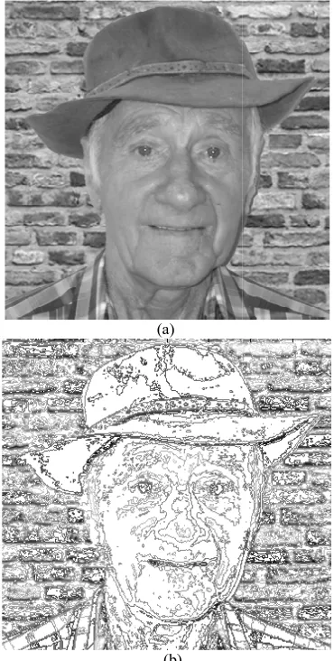
For instance, Figure 1(a) shows the origina (4002) whereas Figure 1(b) is the corresponding contour nodes using line se example, the contour increments in Figure between 0 and 220 grey-scale values or colo bilinear interpolation was used to determin (Watson, 1992).
(a)
(b) Figure 1. (a) The original image of Peter.tif
is a contour representation of (a) for contour 8 grey-scale values.
is used by an image
many grey levels in the pixel values of 20 (within a range of ns. This indicates a s (Cunha et al. 2006) ng between pixels to a contour having the
al image of Peter.tif
results of joining egments. By way of
e 1(b) is 8, ranging ours. In this instance, ne the contour nodes
f (4002), whereas (b) r increments equal to
In the interest of reducing to a min contour vertices, and thus m transmission time, it is often poss using fewer line segments. It is im sufficient details so as to portray minute wavers and concavities. I image will contain contour portion (i.e. straight regions) and portions (i.e. curved regions) as shown in F
A variation of the basic contour
variable line segment boundary r
can be used to better represent sm without using small line segme description.
Therefore, this technique can be contours as it combines multiple them with a single longer segmen that have small direction changes. nodes are covered by a single line contour direction occurs. The nod this process may be recovered if r process.
This way, the line segments of a g record multiple short line segmen the contour direction change only of the line segment approach is car line segment contouring operation that are sufficiently short so as t required to reconstruct an original
Then, the angles of each pair of compared. Where the directional a the two lines segments are comb segment representing their combi (see Figure 2(b)). The end re representation that can be signif maintaining a high level of accurac
Figure 2. (a) A contour often con and regions of great change and ( description combines adjoining co direction angles (after Baxes, 1994
Another technique which may a nodes from the reconstruction pr these contours occupy and the sh their centroids (Bonham-Carter, 2 offer the best statistical constra contour (and its nodes) is very si could be removed.
Also, within any group of at least may possible to test for redund
nimum the number of nodes or minimise data storage and
sible to represent the contours mportant however, to maintain y important features such as In most real world cases, an ns with little direction changes
with a lot of direction change Figure 2(a).
ring approach, referred to as
representation (Baxes, 1994) mall contour segments changes ents throughout the contour
used to remove nodes from e line segments and replaces nt over portions of the contour
A variable number of contour e segment, depending on how des that are eliminated during required in the reconstruction
given contour will not unduly nts (and thereby nodes) where y a little. The implementation rried out by first performing a n, using line segment lengths to contain the contour details
raster image.
f adjoining line segments are angles are similar or identical, bined to create a single line ined length and overall angle esult is a contour segment ficantly more concise, while cy.
ntain regions of little change (b) The variable line segment ontour segments with similar 4)
assist in removing redundant ocess is to compare the area horter and longest distance to 2006). These parameters may aint for deciding whether a
imilar to another and thereby
three close nested contours it dant nodes by removing the International Archives of the Photogrammetry, Remote Sensing and Spatial Information Sciences, Volume XXXIX-B3, 2012
middle contour and interpolate and/or diffuse between the other two. However, this process may have the disadvantage of smoothing and/or distorting particular high frequency (sudden changes of brightness values within an image) information necessary for a more accurate reconstruction of the original image.
3. ENCODING 3D DATA POINTS
For easy extraction, processing and transmission over a digital link, the contours data was encoded and saved in an ASCII file (i.e. txt). This file contains a two-row matrix where each contour line defined in the matrix begins with a column that defines the value of the contour line and the number of (x,y) vertices in the contour line.
The remaining columns contain the data for the (x,y) pairs. The x, y values are stored to the first decimal place and separated by a point. In the coding shown below 120 is the grey-scale intensity of a selected contour and the contour line is formed by 7 vertices. The x coordinate of the vertices are in the top row (i.e. 18.2 17.2...14.7) whereas the corresponding y coordinates are placed in the bottom row (i.e. 110 109...93.2)
120 18.2 17.2 17 17.3 17.1 15.7 14.7
7 110 109 108 99.5 97 95 93.2
Additional tests are presently being undertaken to ascertain the use of binary files (as compared to ASCII .txt file) as a way to further reduce memory requirements and speed of transmission of contour data.
4. FROM 3D POINTS TO PIXELS
In this gridding process contours nodes are projected or mapped on a uniformly spaced grid. Depending on the final resolution required, this grid may be selected so as to create pixels in x and y corresponding to the original input image. To determine the pixel brightness which would exist at the intersections of a regular grid using randomly spaced 3D node locations, several interpolators may be used depending on the application and accuracy requirements.
There exist several interpolation schemes available for this task. Estimations of nearly all spatial interpolation methods can be represented as weighted averages of sampled data (De Jong and van der Meer, 2004). They all share the same general estimation formula as shown in equation 1:
Where Ž is the estimated value of an attribute at the point of interest x0, z is the observed value at the sampled point xi, λiis the weight assigned to the sampled point, and n represents the number of sampled points used for the estimation (Webster and Oliver, 2001).
In this work the interpolation process is an estimation process which determines the pixel brightness which would exist on the intersections of a regular grid using the randomly spaced nodes of contours. Several local interpolators may be used depending on the application and accuracy requirements. The method used in this work is referred to as cubic splines. A brief explanation follows.
The splines consist of polynomials with each polynomial of degree n being local rather than global. The polynomials describe pieces of a line or surface (i.e. they are fitted to a small number of data points exactly) and are fitted together so that they join smoothly (Burrough and McDonnell, 1998; Webster and Oliver, 2001). The places where the pieces join are called knots. The choice of knots is arbitrary and may have an important impact on the estimation (Burrough and McDonnell, 1998). For degree n = 1, 2, or 3, a spline is called linear, quadratic or cubic respectively.
In the ensuing tests, cubic splines were selected as they are very useful for modeling arbitrary functions (Venables and Ripley, 2002) and are used extensively in computer graphics for free form curves and surfaces representation (Akima, 1996).
5. TESTS AND RESULTS
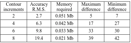
Table 1 shows the results of a first test aimed at determining the degree of accuracy and memory storage requirements to be expected when reproducing a digital image from scattered contour nodes. The figures are based on the Peter.tif (4002) in Figure 1(a). The R.M.S. (Spiegel and Stephens, 1999) is random standard error of the differences of grey-scale values between the original Peter.tif and the same image reconstructed using the nodes for contour increments ranging between 2 and 8.
The figures in Table 1 show a linear degradation of the R.M.S. as the contour interval is increased. The table also illustrates the amount of memory required to store the contour nodes needed for the reconstruction of Peter. As expected, as the contour interval increases, the memory requirement decreases at the expense of image quality.
Contour increments
Accuracy R.M.S.
Memory required
Maximum difference
Minimum difference
2 2.7 0.051 Mb 5 7
4 6.3 0.042 Mb 17 27
6 9.8 0.033 Mb 33 30
8 19.4 0.021 Mb 39 42
Table 1. Accuracy and memory requirements needed to reconstruct the original image of the Peter using contour increments between 2 and 8 grey-scale intensity values.
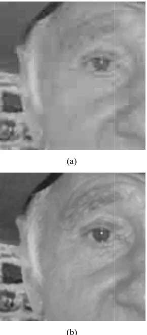
By way of comparison, the .txt file needed to store the x and y coordinates of the nodes necessary to reproduce Peter (for contour increment of 6 grey-scale values) used approximately the same amount of memory of a JPEG compressed (0.029 Mb) version of the same image for a compression ratio of 7:1, while reproducing a more accurate image with improved visual details (see Figure 3).
In Figure 3, the difference in visual quality between Peter
reconstructed with contour data (Figure 3(c)) and the corresponding JPEG image (Figure 3(b)) is evident. Indeed, the blocking effects, typical of a lossy JPEG protocol, were almost completely eliminated.
In addition, the maximum and minimum differences of pixel intensity values resulting from subtracting the JPEG version of
Peter from the original Peter.tif were respectively -36 and +44 grey-scale values with an R.M.S. equal to +/-35. By contrast, the contour approach produced maximum and minimum (1)
differences equal to -33 and +30 respectivel +/- 9.8 pixel grey-scale intensity values.
(a)
(b)
Figure 3. (a) A JPEG version (section on compression ratio of 7:1 and (b) the same using the contour nodes for a contour increm
The proposed compression process was furt image of the lake (4002) and the aerial vie Figure 4 and Figure 5 respectively.
The maximum and minimum differences values resulting from subtracting the JPEG v from the original lake.tif were respectively scale values with an R.M.S. equal to +/-3 contour approach produced maximum and m equal to -35 and +37 respectively with an pixel grey-scale intensity values.
On the other hand, the maximum and mini pixel intensity values resulting from sub version of aerial.jpeg view from the original respectively -35 and +47 grey-scale valu equal to +/-35. By contrast, the contour maximum and minimum differences equ respectively with an R.M.S. of +/- 7.8 pixel values.
ly with an R.M.S. of
nly) of Peter for a image reconstructed ment equal to 5.
ther tested using the ew (4002) shown in
s of pixel intensity version of lake.jpeg
y -39 and +51 grey-38. By contrast, the minimum differences R.M.S. of +/- 10.3
imum differences of btracting the JPEG l aerial view.tif were ues with an R.M.S.
approach produced ual to -31 and +42 l grey-scale intensity
Figure 5. The original ima
Figure 5. The original image
Contour increments
Accuracy R.M.S.
Memor require
2 3.7 0.172 M
4 7.3 0.076 M
6 10.6 0.064 M
8 20.5 0.043 M
Table 2. Accuracy and memo reconstruct the original image of l
between 2 and 8 grey-scale intensi
Contour increments
Accuracy R.M.S.
Memor require
2 3.1 0.151 M
4 6.8 0.062 M
6 8.8 0.059 M
8 18.4 0.041 M
Table 3. Accuracy and memo reconstruct the original image o increments between 2 and 8 grey-s
age of lake.tif (4002).
of aerial view.tif (4002).
ry d
Maximum difference
Minimum difference
Mb 6 8
Mb 23 29
Mb 35 34
Mb 39 46
ory requirements needed to
lake using contour increments ty values
ry d
Maximum difference
Minimum difference
Mb 7 8
Mb 21 31
Mb 37 33
Mb 39 44
ory requirements needed to of aerial view using contour
scale intensity values. International Archives of the Photogrammetry, Remote Sensing and Spatial Information Sciences, Volume XXXIX-B3, 2012
6. COLOUR IMAGES
When processing colour images, the same concepts above hold true. However, instead of a single grey-scale intensity value, colour digital images have pixels that are generally quantised using three components (i.e. Red, Green and Blue). In general, all image processing operations can be extended to process colour images simply by applying them to each colour component (Bovik, 2007).
Each of the three RGB components are processed, encoded and reconstructed separately as if they were three different grey scale images (Duperet, 2002). The results of the three reconstructions are then merged or fused to recreate the original colour image. In terms of image quality (R.M.S.) memory requirements the results from the contouring approach, for the same classes of images (i.e. faces, landscapes and aerial views), were similar to those obtained from the grey-scale imagery described above.
7. CONCLUSIONS
• Generating contour nodes from digital images involves assigning coordinates values to pixels in the raster format, and interpolating between the pixels to find the coordinates of points in the path of a contour having the same grey-scale intensity value. This enables the contour nodes to be found to sub-pixel accuracy if required.
• The conversion of certain classes of digital images into contour maps may be used to compress and reconstruct images in pixel format that are more accurate and with improved visual details than JPEG compressed versions of the same image, while requiring similar memory space for storage and speed of transmission over digital links.
• For the images investigated in this work, the contour approach to image compression requires contour data to be filtered and discriminated from the reconstruction process.
• Spline interpolation was used to reconstruct digital images from the nodes of their contour representations. The process involves determining the pixel intensity value which would exist at the intersections of a regular grid using the nodes of randomly spaced contours.
• Refinements to the proposed method are being undertaken to increase the accuracy achievable for a variety of scenes and dynamic ranges (including bi-tonal imagery).
• More research is required to assess the accuracy of the compression process in the presence of added random noise, a variety of image scenes with various levels of details and/or video imagery.
• Further tests are required to determine whether a binary coding of the contour data may have an impact on memory requirements.
REFERENCES
Akima, H., 1996. Algorithm 761: scattered-data surface fitting that has the accuracy of a cubic polynomial. ACM Transactions on Mathematical Software, 22: 362-371 pages.
Baxes, G. A., 1994. Digital Image Processing: Principles and Applications. John Wiley, Chichester. 452 pages.
Bonham-Carter G. F., 2006. Geographic information systems for geoscientists: modelling with GIS. Vol. 13 of Computer Methods in the Geosciences. Elsevier, Butterworth-Heinemann. 398 pages.
Bovik A., 2007. Handbook of Image and Video Processing. Elsevier Academic Press. Al Bovik editor. 972 pages.
Burrough, P.A. and McDonnell, R.A., 1998. Principles of Geographical Information Systems. Oxford University Press, Oxford, 333 pages.
Cunha A. L., Zhou J. and Do M. N., 2006. The Non-subsampled Contourlet Transform: Theory, Design, and Applications” IEEE Transactions on Image Processing, VOL. 15, NO. 10, October.
De Jong S. M. and van der Meer F.D., 2004. “Remote Sensing Image Analysis Including the Spatial Domain”, Kluwer Academic Publishers, pp. 360.
Duperet, A., 2002. “Image Improvements, Chapter 2, Digital Photogrammetry.” Michel Kasser and Yves Egels editors, Taylor & Francis Publishers. p.p. 351: 79-100.
Elder J. H. and Goldberg R. M. 2001. Image Editing in the Contour Domain. IEEE Transactions on Pattern Analysis and Machine. Vol 23 No. 3.
Elder J.H. and Zucker S. W. 1998. Local Scale Control for Edge Detection and Blur Estimation." IEEE Transactions on Pattern Analysis and Machine Intelligence. col.20, No. 7.
Gonzalez R. C. and Woods R. E., 2008. Digital image processing. Prentice Hall, 954 pages.
Russ C. J., 2002. The Image Processing Handbook. CRC Press; 4th edition. 732 pages.
Smith M. Goodchild F. and Longley P.A., 2009. Geospatial Analysis: A Comprehensive Guide to Principles, Techniques and Software Tools. 3d. Edition. The Winchelsea Press. 560 pages.
Spiegel M. R., Stephens L, 1999. Theory and Problems of Statistics, Schaum’s Outline Series, McGraw-Hill Book Company. 556 pages.
Venables, W.N. and Ripley, B.D., 2002. Modern Applied Statistics with S-Plus. Springer-Verlag, New York, 495 pp.
Vasilyev, S. V. 1999. A Contour-Based Image Compression for Fast Real-Time Coding. in ASP Conf. Ser., Vol. 172, Astronomical Data Analysis Software and Systems VIII, eds. D. M. Mehringer, R. L. Plante, & D. A. Roberts (San Francisco: ASP).
Wang S., Ge F. and Liu T. 2006. Evaluating edge detection through boundary detection. EURASIP Journal on Applied Signal Processing, vol. 2006, pages 1–15.
Watson D. F. 1992. “Contouring: A Guide to the Analysis and Display of Spatial Data”. Pergamon Press. New York. 321 pages.
Weeks, A. R., 1996. Fundamentals of Electronic Image Processing. SPIE Optical Engineering Press, Bellingham, Washington. 570 pages.
Webster, R. and Oliver, M., 2001. Geo-statistics for Environmental Scientists. John Wiley & Sons, Ltd, Chichester, 271 pages.