DYNAMICS BASED CONTROL OF A SKID STEERING MOBILE ROBOT
Osama Elshazly1, Hossam S. Abbas2, and Zakarya Zyada3
1Mechatronics and Robotics Eng. Dept., Egypt-Japan University of Science and Technology (E-JUST), Qesm Borg Al Arab, Alexandria, 21934, Egypt
2Electrical Eng. Dept., Faculty of Engineering, Assiut University, Al Hamraa Ath Thaneyah, Qesm Than Asyut, Assiut, 71515, Egypt
3Faculty of Mechanical Engineering (FKM), Universiti Teknologi Malaysia, 81310 Johor, Malaysia. (”On-leave” Mechanical Power Engineering, Tanta University, 31511 Tanta, Egypt.) E-mail: [email protected], [email protected]2, [email protected]3
Abstract
In this paper, development of a reduced order, augmented dynamics-drive model that combines both the dynamics and drive subsystems of the skid steering mobile robot (SSMR) is presented. A Linear Quadratic Regulator (LQR) control algorithm with feed-forward compensation of the disturbances part included in the reduced order augmented dynamics-drive model is designed. The proposed controller has many advantages such as its simplicity in terms of design and implementation in comparison with complex nonlinear control schemes that are usually designed for this system. Moreover, the good performance is also provided by the controller for the SSMR comparable with a nonlinear controller based on the inverse dynamics which depends on the availability of an accurate model describing the system. Simulation results illustrate the effectiveness and enhancement provided by the proposed controller.
Keywords: Skid Steering Mobile Robots, Reduced order model, Linear Quadratic Regulator, Feed-Forward Compensation, Inverse Dynamics.
Abstrak
Dalam paper ini, pengembangan reduced order, augmented model dynamics-drive yang
mengga-bungkan kedua dinamika dan subsistem drive dari skid steering mobile robot (SSMR) ditampilkan.
Sebuah algoritma kontrol Linear Quadratic Regulator (LQR) dengan kompensasi feed-forward dari
disturbances part termasuk dalam reduced orderaugmented model dynamics-drive dirancang.
Pengen-dali yang diusulkan memiliki banyak keuntungan seperti kesederhanaan dalam hal desain dan imple-mentasi dibandingkan dengan skema kontrol nonlinear kompleks yang biasanya dirancang untuk sistem ini. Selain itu, kinerja yang baik juga disediakan oleh pengendali untuk SSMR sebanding dengan
pe-ngendali nonlinear berdasarkan dinamika inverse yang tergantung pada ketersediaan dari model yang
akurat yang menggambarkan sistem. Hasil simulasi menggambarkan efektivitas dan peningkatan oleh pengendali yang diusulkan.
Kata Kunci: Skid Steering Mobile Robots, Reduced order model, Linear Quadratic Regulator, Kompensasi Feed-Forward, Dinamika Inverse.
1. Introduction
Nowadays, mobile robotics constitute an attractive research field with a high potential for practical ap-plications. Skid steering mobile robots (SSMR) are widely used as outdoor mobile robots. Simple and robust mechanical structure, faster response, high maneuverability, strong traction, and high mobility make SSMR to be suitable for many applications such as loaders, farm machinery, mining and mili-tary applications [1][2]. Due to complex kinematic constraints and wheel/ground interactions, consi-dering the dynamical model and designing a proper controller for skid-steering mobile robots (SSMR)
are challenging tasks. For the topic of skid steering mobile robots modelling and control, several search papers have been published to cover this re-search field. The stability of wheeled skid steering mobile robots has been studied using model based nonlinear control techniques by explicitly conside-ring dynamics and drive models [3-5].
simpli-fied dynamic model for wheeled skid steering mo-bile robots is considered using an online adaptive control [8]. A trajectory tracking control were pre-sented in [9] to control a wheeled skid-steering mo-bile robot moving on a rough terrain based on dif-ferent control methods such as practical fuzzy la-teral control, longitudinal control and sensor pantilt control; the authors used ADAMS and MATLAB co-simulation platform to assess these control laws. In [10] [11], a thorough dynamic analysis of a skid-steered vehicle has been introduced; this analysis considers steady-state (i.e. constant linear and ang-ular velocities) dynamic models for circang-ular motion of tracked vehicles.
The control system design for such SSMR dy-namics and drive subsystems was done indepen-dently without considering the combination bet-ween dynamic and drive model. Moreover, the ro-bot motor voltages/torques may be the true control inputs of some mobile robots. In other words, the low level control of such mobile robot may be es-sential for trajectory tracking problem to consider robot dynamics. Therefore, the main contribution in this paper is to design a dynamics-based control-ler to control the augmented dynamics-drive model which has the inputs of motors voltages and the outputs of robots are the longitudinal and angular velocities.
In this paper, a reduced order, augmented dy-namics-drive model that combines both the dyna-mics and drive subsystems of the SSMR based on [3] is developed. Then, a Linear Quadratic Regula-tor (LQR) with feed-forward compensation of the disturbances part included in the reduced order augmented dynamics-drive model is developed. For comparison, an inverse dynamics controller is designed. The main advantage of the proposed LQR controller is simplicity of design and expe-rimental implementation in comparison with non-linear controllers which are highly complex for im-plementation. The two controllers are used for a re-ference tracking of SSMR.
The remaining of the paper is organized as fo-llows: A reduced order augmented dynamics-drive model of SSMR is presented in a systematic way in section 2. Section 2 is also devoted to present the development of the controller using LQR with feed forward compensation for the system. An inverse
dynamics controller is presented to ensure robust-ness to the nonlinearities of dynamical model. Sec-tion 3 is dedicated for extensive simulaSec-tion results considering trajectory tracking problem. Conclusi-ons and ideas for future work are given in Section 4. Finally, acknowledgments and references com-plete the paper.
2. Methods
Robot Model
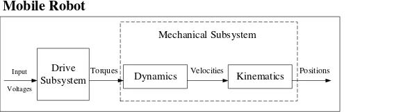
In this subsection, the dynamics mathematical des-cription of an SSMR moving on a planar surface is reviewed. The mobile robot mathematical model [3] can be divided into three parts: kinematics, dy-namics and drive subsystems, see Figure 1. In this paper, we focus on the first two blocks, i.e., the dri-ve and dynamics subsystems, and we use them for reference tracking control of both the linear and angular velocities.
Model of Dynamics Subsystem
The dynamics effects play an important role in SS-MR vehicles. Such dynamics consider the forces and torques required to cause the robot motion. Considering forces and torques is important in mo-bile robot control to follow a desired trajectory.
Moreover, dynamics consider the wheel grou-nd interactions which affect the performance of the SSMR vehicles. So, this subsection is dedicated for the dynamics properties of the SSMR moving on a Drive
Subsystem Dynamics Kinematics
Input Voltages
Torques Velocities Positions
Mechanical Subsystem Mobile Robot
Figure 1. An electrically driven mobile robot decomposition
planar surface as shown in Figure 2 to be described [3][4]. It is assumed that the mass distribution of the vehicle is homogeneous, kinetic energy of the wheels and drives is neglected and detailed deriva-tions of the tire reladeriva-tions is omitted and the reader can return to [3] for more details.
Using the Euler-Lagrange principle with La-grange multipliers to include non-holonomic cons-traints, the dynamics equation of the robot can be obtained. The planar motion of SSMR allows us to assume that the potential energy of the robot is
𝑃𝑃𝑃𝑃(𝑞𝑞) = 0. Therefore the Lagrangian L of the sys-tem equals the kinetic energy as given by equation(1):
𝐿𝐿(𝑞𝑞,𝑞𝑞̇) =𝑇𝑇(𝑞𝑞,𝑞𝑞̇) (1)
The following equation(2) can be developed if the kinetic energy of the vehicle is considered and the energy of rotating wheels is neglected:
𝑇𝑇(𝑞𝑞,𝑞𝑞̇) =12𝑚𝑚𝑣𝑣𝑇𝑇𝑣𝑣+1
2𝐼𝐼𝑤𝑤2 (2)
where 𝑚𝑚 and 𝐼𝐼 represent the mass of the robot and moment of inertia of the robot about the COM, respectively. Equation(2) can be rewritten in the following equation(3) (since 𝑣𝑣𝑇𝑇𝑣𝑣=𝑣𝑣
𝑥𝑥2+ 𝑣𝑣𝑦𝑦2=𝑋𝑋̇2+𝑌𝑌̇2).
𝑇𝑇(𝑞𝑞,𝑞𝑞̇) =1
2𝑚𝑚(𝑋𝑋̇2+𝑌𝑌̇2) +
1
2𝐼𝐼𝜃𝜃̇2 (3)
The inertial forces can be obtained after cal-culating the partial derivative of kinetic energy and its time-derivative as given by equation(4).
where:
𝑀𝑀=�
𝑚𝑚 0 0
0 𝑚𝑚 0 0 0 𝐼𝐼
� (5)
Based on Fig.3, the generalized resistive for-ces can be calculated as the following equation(6).
𝑅𝑅(𝑞𝑞̇) = [𝐹𝐹𝑟𝑟𝑥𝑥(𝑞𝑞̇) 𝐹𝐹𝑟𝑟𝑦𝑦(𝑞𝑞̇) 𝑀𝑀𝑟𝑟(𝑞𝑞̇)]𝑇𝑇 (6)
such that, 𝐹𝐹𝑟𝑟𝑥𝑥(𝑞𝑞̇) and 𝐹𝐹𝑟𝑟𝑦𝑦(𝑞𝑞̇) are the resultant forces expressed in the inertial frame which can be calcu-lated as given by equation(7) and equation(8).
𝐹𝐹𝑟𝑟𝑥𝑥(𝑞𝑞̇) = cos𝜃𝜃 � 𝐹𝐹𝑠𝑠𝑠𝑠(𝑣𝑣𝑠𝑠𝑥𝑥) 4
𝑠𝑠=1
−sin𝜃𝜃 � 𝐹𝐹𝑙𝑙𝑠𝑠�𝑣𝑣𝑠𝑠𝑦𝑦�
4
𝑠𝑠=1
(7)
𝐹𝐹𝑟𝑟𝑦𝑦(𝑞𝑞̇) = sin𝜃𝜃 � 𝐹𝐹𝑠𝑠𝑠𝑠(𝑣𝑣𝑠𝑠𝑥𝑥) 4
𝑠𝑠=1
+ cos𝜃𝜃 � 𝐹𝐹𝑙𝑙𝑠𝑠�𝑣𝑣𝑠𝑠𝑦𝑦�
4
𝑠𝑠=1
(8)
Also, the resistant moment around the center of mass 𝑀𝑀𝑟𝑟(𝑞𝑞̇) can be obtained as given by equation (9).
𝑀𝑀𝑟𝑟(𝑞𝑞̇) =−𝑎𝑎 � 𝐹𝐹𝑙𝑙𝑠𝑠�𝑣𝑣𝑠𝑠𝑦𝑦�
𝑠𝑠=1,4 +𝑏𝑏 �𝑠𝑠=2,3𝐹𝐹𝑙𝑙𝑠𝑠�𝑣𝑣𝑠𝑠𝑦𝑦�
+𝑐𝑐 �− � 𝐹𝐹𝑠𝑠𝑠𝑠(𝑣𝑣𝑠𝑠𝑥𝑥) 𝑠𝑠=1,2
+� 𝐹𝐹𝑠𝑠𝑠𝑠(𝑣𝑣𝑠𝑠𝑥𝑥)
𝑠𝑠=3,4 �
(9)
such that 𝐹𝐹𝑠𝑠𝑠𝑠results from the rolling resistant mo-ment 𝜏𝜏𝑟𝑟𝑠𝑠 as shown in Figure 4 and 𝐹𝐹𝑙𝑙𝑠𝑠 denotes the lateral reactive force. 𝐹𝐹𝑠𝑠𝑠𝑠 and 𝐹𝐹𝑙𝑙𝑠𝑠can be considered as wheel friction forces and can be described as given by equation(10).
𝐹𝐹𝑠𝑠𝑠𝑠=𝜇𝜇𝑠𝑠𝑠𝑠𝑠𝑠𝑚𝑚𝑚𝑚 sgn(𝑣𝑣𝑠𝑠𝑥𝑥)
𝐹𝐹𝑙𝑙𝑠𝑠 =𝜇𝜇𝑙𝑙𝑠𝑠𝑠𝑠𝑚𝑚𝑚𝑚 sgn (10)
where 𝜇𝜇𝑠𝑠𝑠𝑠𝑠𝑠 and 𝜇𝜇𝑙𝑙𝑠𝑠𝑠𝑠 denote the coefficients of the longitudinal and lateral friction forces. 𝑚𝑚is the gra-vity of acceleration. The active force 𝐹𝐹𝑠𝑠is linearly dependent on the wheel control input 𝜏𝜏𝑠𝑠by the in-verse of the wheel radius (r) given by equation(11).
𝐹𝐹 𝜏𝜏𝑖𝑖
inertial frame as the following equation(12).
𝐹𝐹𝑥𝑥= cos𝜃𝜃 ∑4𝑠𝑠=1𝐹𝐹𝑠𝑠 (12)
𝐹𝐹𝑦𝑦= sin𝜃𝜃 ∑ 𝐹𝐹4𝑠𝑠=1 𝑠𝑠
The active torque around the COM is calcu-lated as defined in equation(13).
𝑀𝑀=𝑐𝑐(−𝐹𝐹1− 𝐹𝐹2+𝐹𝐹3+𝐹𝐹4) (13)
In consequence, the vector F of active forces has the following equation(14).
𝐹𝐹= [𝐹𝐹𝑥𝑥 𝐹𝐹𝑦𝑦 𝑀𝑀]𝑇𝑇 (14) Using equations(11) to equation(13), and assuming that the radius of each wheel is the same, we get equation(15).
𝐹𝐹=1
𝑟𝑟�
cos𝜃𝜃 ∑ 𝐹𝐹4𝑠𝑠=1 𝑠𝑠 sin𝜃𝜃 ∑4𝑠𝑠=1𝐹𝐹𝑠𝑠 𝑐𝑐(−𝐹𝐹1− 𝐹𝐹2+𝐹𝐹3+𝐹𝐹4)
� (15)
A new torque control input τ is defined for notation simplification as equation(16).
𝜏𝜏=�𝜏𝜏𝜏𝜏𝐿𝐿
𝑅𝑅�=�
𝜏𝜏1+𝜏𝜏2
𝜏𝜏3+𝜏𝜏4� (16)
where 𝜏𝜏𝐿𝐿 and 𝜏𝜏𝑅𝑅 denote the torques produced by the wheels on the left and right sides of the vehicle, res-pectively. Using equation(15) and equation (16), we can obtain the following equation(17).
𝐹𝐹=𝐵𝐵(𝑞𝑞)𝜏𝜏 (17)
such that 𝐵𝐵is the input transformation matrix defi-ned as equation(18).
𝐵𝐵=1𝑟𝑟�
cos𝜃𝜃 cos𝜃𝜃 sin𝜃𝜃 sin𝜃𝜃
−𝑐𝑐 𝑐𝑐 � (18)
The following dynamics model (equation (19)) is obtained using equation(4), equation(6) and equation(17).
𝑀𝑀(𝑞𝑞)𝑞𝑞̈+𝑅𝑅𝑞𝑞̈=𝐵𝐵(𝑞𝑞) 𝜏𝜏 (19) A velocity constraint can be considered in order to complete the kinematic model as equation(20).
𝑣𝑣𝑦𝑦+𝑥𝑥𝐼𝐼𝐼𝐼𝑅𝑅𝜔𝜔= 0 (20)
Equation(20) describes a non-holonomic constraint which can be written in the Pfaffian form as equa-tion(21).
[−sin𝜃𝜃 cos𝜃𝜃 𝑥𝑥𝐼𝐼𝐼𝐼𝑅𝑅][𝑋𝑋̇ 𝑌𝑌̇ 𝜃𝜃̇]𝑇𝑇=𝐴𝐴(𝑞𝑞)𝑞𝑞̇= 0 (21) The equation that describe the kinematics of the robot is given by [3]:
𝑞𝑞̇=�𝑋𝑋̇𝑌𝑌̇
𝜃𝜃̇�
=�
cos𝜃𝜃 𝑥𝑥𝐼𝐼𝐼𝐼𝑅𝑅sin 𝜃𝜃 sin𝜃𝜃 −𝑥𝑥𝐼𝐼𝐼𝐼𝑅𝑅cos𝜃𝜃
0 𝑐𝑐1
� �𝑣𝑣𝜔𝜔𝑥𝑥�=𝑆𝑆(𝑞𝑞)𝜂𝜂 (22)
here 𝜂𝜂 = [𝑣𝑣𝑥𝑥 𝜔𝜔]𝑇𝑇, 𝑣𝑣𝑥𝑥 is the longitudinal velo-city, 𝜔𝜔is the angular velocity of the robot, 𝜏𝜏is the torque control input, and 𝑞𝑞 = [𝑋𝑋 𝑌𝑌 𝜃𝜃]𝑇𝑇 repre-sents the generalized coordinates of the center of mass (COM) of the robot, i.e., the COM position, with 𝑋𝑋 and 𝑌𝑌; and 𝜃𝜃is the orientation of the local coordinate frame with respect to the inertial frame. Equation(19) describes the dynamics of a free body only and does not include the non-holonomic constraint described by equation(21), so a constra-int has to be imposed on equation(19). A vector of Lagrange multipliers, 𝜆𝜆, is introduced to include the non-holonomic constraint into the dynamics equation as the following equation(23).
𝑀𝑀(𝑞𝑞)𝑞𝑞̈+𝑅𝑅𝑞𝑞̈=𝐵𝐵(𝑞𝑞)𝜏𝜏+𝐴𝐴𝑇𝑇(𝑞𝑞)𝜆𝜆 (23)
It would be more suitable to express equation (23) as a function of the internal velocity vector 𝜂𝜂 for control purposes. So, by multiplying equation (23) by 𝑆𝑆𝑇𝑇(𝑞𝑞) from the left, we can obtain the fol-lowing equation(24).
Figure 4. Forces acting on a wheel
𝑆𝑆𝑇𝑇(𝑞𝑞) 𝑀𝑀(𝑞𝑞)𝑞𝑞̈+𝑆𝑆𝑇𝑇(𝑞𝑞) 𝑅𝑅𝑞𝑞̈=𝑆𝑆𝑇𝑇(𝑞𝑞) 𝐵𝐵(𝑞𝑞)𝜏𝜏+𝑆𝑆𝑇𝑇(𝑞𝑞) 𝐴𝐴𝑇𝑇(𝑞𝑞)𝜆𝜆 (24)
By taking the time derivative of equation(22), we obtain equation(25).
𝑞𝑞̈=𝑆𝑆̇(𝑞𝑞)𝜂𝜂+𝑆𝑆(𝑞𝑞)𝜂𝜂̇ (25) From equation(22), equation(23), and equa-tion(25), the dynamic equation as introduced in [3] is defined in equation(26).
𝑀𝑀�(𝑞𝑞)𝜂𝜂̇+𝐶𝐶̅(𝑞𝑞̇)𝜂𝜂+𝑅𝑅�(𝑞𝑞̇) =𝐵𝐵�(𝑞𝑞)𝜏𝜏 (26)
The matrices 𝑀𝑀�,𝐶𝐶̅,𝑅𝑅�, and 𝐵𝐵� are given, respecti-vely, by equation(27) to equation(30).
𝑀𝑀�=�𝑚𝑚0 𝑚𝑚𝑥𝑥 0
Equation(26) can be written as the following equa-tion(31).
𝜂𝜂̇=𝑀𝑀�−1(𝑞𝑞)𝐵𝐵�(𝑞𝑞)𝜏𝜏 − 𝑀𝑀�−1(𝑞𝑞)𝐶𝐶̅𝜂𝜂 − 𝑀𝑀�−1(𝑞𝑞)𝑅𝑅�(𝑞𝑞̇) (31) where 𝑀𝑀�is nonsingular for all 𝑞𝑞, 2𝑐𝑐is the vehicle width, and the coordinate of the instantaneous cen-ter of rotation (ICR) is defined as (𝑥𝑥𝐼𝐼𝐼𝐼𝑅𝑅, 𝑦𝑦𝐼𝐼𝐼𝐼𝑅𝑅). Model of Drive Subsystem
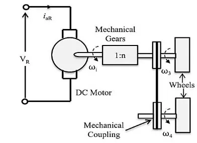
In this subsection, the drive subsystem of an SSMR model is developed. It is assumed that the robot is driven by two DC motors, one at each side, with mechanical gears. Moreover, it is also assumed that there is no slip in the belt which connect each two wheels on each side and there are no nonlinearities in the mechanical coupling in the drive subsystem. In Figure 5, a simplified scheme of the drive on the right side of the robot is depicted. Considering only one drive and assuming that the two motors and gears have the same parameters, the relation bet-ween the torque 𝜏𝜏𝑅𝑅 and voltage 𝑉𝑉𝑅𝑅 can be written as the following equation(32).
𝑉𝑉𝑅𝑅=𝐿𝐿𝑎𝑎𝑑𝑑𝑑𝑑𝑑𝑑𝑖𝑖𝑎𝑎𝑅𝑅+𝑅𝑅𝑎𝑎𝑖𝑖𝑎𝑎𝑅𝑅+𝑛𝑛𝐾𝐾𝑒𝑒𝜔𝜔𝑅𝑅 (33)
where𝐿𝐿𝑎𝑎and 𝑅𝑅𝑎𝑎 denote the series inductance and resistance of the rotors, respectively, 𝐾𝐾𝑒𝑒is the elec-tromotive force, and 𝜔𝜔𝑅𝑅 is the right hand side mo-tor angular velocity.
The left 𝜔𝜔𝐿𝐿 and right 𝜔𝜔𝑅𝑅 sides angular veloci-ties can be obtained from the following equation (34) and equation(35).
𝜔𝜔𝐿𝐿=𝑣𝑣𝑥𝑥−𝑠𝑠𝑐𝑐𝑟𝑟 (34)
𝜔𝜔𝑅𝑅=𝑣𝑣𝑥𝑥+𝑠𝑠𝑐𝑐𝑟𝑟 (35)
In order to obtain the overall model of the two motors of the drive system, Equation(33) can be written as the following equation(36) and equation (37). voltage signals, respectively.
Dynamics-Drive Augmented Model
In previous work, a control law was designed for dynamics and drive models independently. Howe-ver, in this research it is required to design one con-troller for both dynamics and drive models. So, the drive and the dynamics subsystems are combined in one state space representation for such purpose. Substitution from equation(32) into equation(31), gives theis equation(38).
�𝑣𝑣̇𝑥𝑥
𝜔𝜔̇�=𝑛𝑛𝐾𝐾𝑚𝑚𝑀𝑀�−1𝐵𝐵� �𝑖𝑖𝑖𝑖𝑎𝑎𝑅𝑅𝑎𝑎𝐿𝐿� − 𝑀𝑀�−1𝐶𝐶̅ �𝑣𝑣𝜔𝜔� − 𝑀𝑀𝑥𝑥 �−1𝑅𝑅�(38)
presented by the following state space
represent-It may be difficult to design a controller for a system offourth order described by equation(40). So, it will be simpler if the system is reduced to a lower order. The order of the model described by equation(40) can be reduced to 2 by neglecting the motor inductance, i.e. 𝐿𝐿𝑎𝑎= 0. Therefore, equation (33) can be written defined in equation(43).
𝑉𝑉𝑅𝑅=𝑅𝑅𝑎𝑎𝑖𝑖𝑎𝑎𝑅𝑅+𝑛𝑛𝐾𝐾𝑒𝑒𝜔𝜔𝑅𝑅 (43)
From equation(43), we can obtain the current of the motors as equation(44).
�𝑖𝑖𝑎𝑎𝐿𝐿
The motors torque can be calculated as:
�𝜏𝜏𝜏𝜏𝐿𝐿
By using equation(45), the state space repre-sentation of the reduced order overall system can be given by equation(46).
�𝑣𝑣̇𝑥𝑥
Equation(46) can be written in the general form of the state space representation as the following equation(50).
𝑋𝑋̇=𝐴𝐴2(𝑋𝑋)𝑋𝑋+𝐵𝐵2𝑈𝑈+𝐷𝐷2(𝑋𝑋) (50)
where the system states are represented by equation (51).
𝑋𝑋= [𝑣𝑣𝑥𝑥 𝜔𝜔]𝑇𝑇 (51)
The control input vector 𝑈𝑈 is represented by 𝑈𝑈= [𝑉𝑉𝐿𝐿 𝑉𝑉𝑅𝑅]𝑇𝑇= [𝑉𝑉1 𝑉𝑉2]𝑇𝑇.
Finally, we consider D2(X), the last term of equation(50) as a disturbance; this will be neglect-ted in the design of the Linear Quadratic Regulator (LQR) in the next subsection; however, it will be considered in the design of the feed-forward con-troller to overcome its effect on the system as sho-wn below in the next subsection.
Dynamics-Based Controller
Motor voltages/torques may be the true control in-puts of some mobile robots. In other words, the low level control of such mobile robot may be essential for trajectory tracking problem to consider robot dynamics. So, dynamics-based controller is presen-ted to control the augmenpresen-ted dynamics-drive mo-del which has the inputs of motors’ voltages (𝑉𝑉𝐿𝐿 and 𝑉𝑉𝑅𝑅) and the outputs of robot’s velocities (𝑣𝑣𝑥𝑥 and 𝜔𝜔). In this section, two control laws are intro-duced, LQR with feed-forward compensation and inverse dynamics controller to be used for a refe-rence tracking of the augmented dynamics-drive model presented in the previous section.
Linear Quadratic Regulator (LQR)
ob-tain an optimal control law in order to minimize a cost function along the trajectory of a linear sys-tem. Consider the state space representation of a system [12]:
𝑋𝑋̇=𝐴𝐴𝑋𝑋+𝐵𝐵𝑈𝑈 (52)
𝑌𝑌=𝐶𝐶𝑋𝑋 (53)
with 𝑋𝑋(𝑡𝑡)∈ 𝑅𝑅𝑛𝑛, 𝑈𝑈 (𝑡𝑡) ∈ 𝑅𝑅𝑚𝑚 and the initial con-dition is 𝑋𝑋(0). We assume here that all the states are measurable and seek to find a state-variable feedback control law as equation(54).
𝑈𝑈=−𝐾𝐾𝑋𝑋 (54)
that gives desirable closed-loop properties such th-at K is the feedback gain vector. The optimal feedback state regulation minimizes the quadratic cost function defined by equation(55).
𝐽𝐽=1
2∫ (𝑋𝑋𝑇𝑇𝑄𝑄𝑋𝑋+𝑈𝑈𝑇𝑇𝑅𝑅𝑈𝑈)𝑑𝑑𝑡𝑡
∞
0 (55)
where 𝑄𝑄is a symmetric positive semi-definite ma-trix and 𝑅𝑅is a symmetric positive definite matrix. The optimal feedback gain vector can be calculated by equation(56).
𝐾𝐾=𝑅𝑅−1𝐵𝐵𝑇𝑇𝑃𝑃 (56)
where P is the solution of the Algebraic Riccati
Our objective is to design an optimal control law to provide a reference tracking controller of a linearized model of the skid steering mobile robot vehicle using the voltages of the two motors as the inputs to the system. The closed loop reference tracking control system for the SSMR is described by equations (52) and (53). The control law for re-ference tracking LQR controller can be defined as equation(58) [13]:
𝑈𝑈=−𝐾𝐾𝑋𝑋+𝑉𝑉𝑌𝑌𝑑𝑑 (58)
where 𝑉𝑉=−(𝐶𝐶𝑇𝑇(𝐴𝐴 − 𝐵𝐵𝐾𝐾)−1𝐵𝐵)−1 to insure zero steady-state error and 𝑌𝑌𝑑𝑑is the desired output.
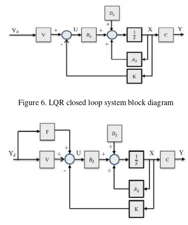
The block diagram that describes the closed loop system for the augmented dynamics-drive model which was described by equation(50) with the LQR control law defined by equation(58) is de-picted in Figure 6.
Feed-Forward Compensation
In the simulation, the term D2(x) of equation(50) is considered as a disturbance; therefore, the system response is tested with and without this term to check its effect. A feed-forward compensation is proposed to overcome the effect of this term.
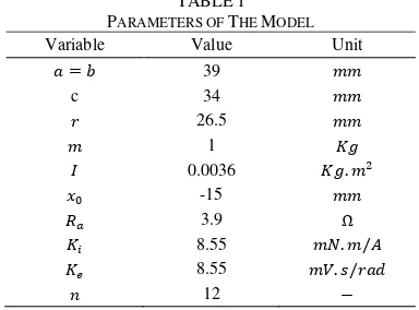
The overall closed-loop block diagram of the system with the LQR controller and the feed-for-ward compensation is depicted in Figure 7, where F is a vector which can be calculated by equation (59).
Figure 6. LQR closed loop system block diagram
Figure 7. LQR with feed-forward compensation.
Figure 8. Inner-outer loop control for inverse dynamics
This vector represents the compensation of the two components of 𝐷𝐷2(𝑥𝑥).
Inverse Dynamics Controller
As presented before, the LQR controller with feed-forward compensation was designed for a linear-ized model of the SSMR and it is more favorable to design a controller for the nonlinear model of the SSMR directly. So, we design an inverse dynamics controller for the nonlinear system model based on the idea presented in [14]. Consider again the SS-MR dynamics model described by equation(50). The idea of inverse dynamics is to seek a non-linear feedback control law described by equation(60).
𝑈𝑈=𝑓𝑓(𝑋𝑋,𝑡𝑡) (60) The block diagram of the scheme of the inverse dy-namics control is shown in Figure 8. Consider a new input to the system 𝑎𝑎𝑞𝑞such the equation(61).
𝑎𝑎𝑞𝑞=𝐴𝐴2(𝑋𝑋)𝑋𝑋+𝐵𝐵2𝑈𝑈+𝐷𝐷2(𝑋𝑋) (61)
By mathematical manipulation (equation(62)) of equation(61), we can obtain the control input 𝑈𝑈as equation(63).
𝑎𝑎𝑞𝑞− 𝐴𝐴2(𝑋𝑋)𝑋𝑋 − 𝐷𝐷2(𝑋𝑋) =𝐵𝐵2𝑈𝑈 (62) 𝑈𝑈=𝐵𝐵2−1(𝑎𝑎𝑞𝑞− 𝐴𝐴2(𝑋𝑋)𝑋𝑋 − 𝐷𝐷2(𝑋𝑋)) (63)
The new control input 𝑎𝑎𝑞𝑞can be given by equation (64).
𝑎𝑎𝑞𝑞=𝑘𝑘(𝑋𝑋 − 𝑋𝑋𝑟𝑟𝑒𝑒𝑟𝑟) (64)
where 𝑘𝑘is the gain to be designed for the controller
and 𝑋𝑋𝑟𝑟𝑒𝑒𝑟𝑟 is the reference system states.
3. Results and Analysis
In this simulation, the dynamic and drive models described by the reduced order model (46) is considered, so the inputs to the system are the two motor voltages 𝑉𝑉1 and 𝑉𝑉2 and the outputs of the sys-tem are the linear velocity 𝑣𝑣𝑥𝑥 and angular velocity
𝜔𝜔. The system parameters applied for simulation are shown in Table 1. In practice, it is difficult to measure 𝑥𝑥𝐼𝐼𝐼𝐼𝑅𝑅 value, so it is assumed here to be equation(65) [3] [4].
𝑥𝑥𝐼𝐼𝐼𝐼𝑅𝑅 =𝑐𝑐𝑐𝑐𝑛𝑛𝑐𝑐𝑡𝑡𝑎𝑎𝑛𝑛𝑡𝑡=𝑥𝑥0 𝑥𝑥0𝜖𝜖 (−𝑎𝑎,𝑏𝑏) (65)
where 𝑎𝑎 and 𝑏𝑏 are positive kinematic parameters of the robot depicted in Figure 2.
LQR with Feed-Forward Compensation
Controller Results
For the LQR controller, the matrices 𝑄𝑄 and 𝑅𝑅, whi-ch are described in equation(57), are whi-chosen by trial and error to be equation(66).
𝑄𝑄=�0.1 0
0 0� 𝑅𝑅=�
1 0
0 0� (66)
In simulation, we test three cases for the sys-tem. Firstly, we assume that the system described by equation(50) is without the disturbance 𝐷𝐷2(𝑥𝑥) term as shown in Figure 9. Secondly, this term
𝐷𝐷2(𝑥𝑥) is added to the system as depicted in Figure
6 to check its effect on the response and asses the controller performance. Finally, the feed-forward compensation part is included as shown in Figure 7 to overcome the effect of the disturbance part
𝐷𝐷2(𝑥𝑥).
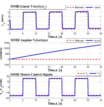
Figure 10 shows the system response to a square reference for both the linear and angular velocities. The system can track the desired inputs quickly and without any overshoot. Also, Figure 10 provides the control signals of the system motors and it is obvious that the control signals are in the limits of the maximum motor voltages (±24V DC). In order to demonstrate the effectiveness of the controller, the term D2(x) is added to the system and the system response and control signals are shown in Figure 11. It can be shown that the system is affected by this part which destabilizes the angu-lar velocity output.
In order to overcome the effect of D2(x), the feed-forward compensation is added to the control-ler. The system response and control signals are shown in Figure 12. It is shown that the system can again track the desired references. Moreover, we see that the control signals are different from those that are depicted in Figure 10 and Figure 11 as the control law is changed, see Figure 7.
From the above analysis, the simulation re-sults illustrate that the LQR performance is
enhan-TABLE1 PARAMETERS OF THE MODEL
Variable Value Unit
𝑎𝑎=𝑏𝑏 39 𝑚𝑚𝑚𝑚
c 34 𝑚𝑚𝑚𝑚
𝑟𝑟 26.5 𝑚𝑚𝑚𝑚
𝑚𝑚 1 𝐾𝐾𝑚𝑚
𝐼𝐼 0.0036 𝐾𝐾𝑚𝑚.𝑚𝑚2
𝑥𝑥0 -15 𝑚𝑚𝑚𝑚
𝑅𝑅𝑎𝑎 3.9 Ω
𝐾𝐾𝑠𝑠 8.55 𝑚𝑚𝑚𝑚.𝑚𝑚/𝐴𝐴
𝐾𝐾𝑒𝑒 8.55 𝑚𝑚𝑉𝑉.𝑐𝑐/𝑟𝑟𝑎𝑎𝑑𝑑
ced for the linearized model; however, the stability and tracking of the reference input may not be gua-ranteed if this controller is applied to the nonlinear system as it was applied to a linearized model with disturbance term only and the stability and tracking is not guaranteed.
Inverse Dynamics Controller Results
Next, we apply the inverse dynamics controller to the nonlinear system described by equation(50)
inverse dynamics controller that can deal with non- linear systems. Also, the two control signals are wi-thin the limits of the motor voltages. But, it is clear from the inverse dynamics controller design that an accurate model of the nonlinear system is needed as its proper design depends on the system matri-ces. Finally, it should be noted that the inverse dy-namics controller is applied to the nonlinear model of the SSMR directly while the LQR with the feed-forward compensation is applied to a linearized model of the system.
4. Conclusion
An LQR with feed-forward compensation algori-thm is presented in this paper for controlling a
Figure 12. System response with feed-forward compensation
Figure 13. System response with an inverse dynamic controller
Figure 10. System response (without the nonlinear term D2(x))
ve tracking accuracy and overcome effects of non- linearities. For comparison, an inverse dynamics controller is designed. The LQR controller with the feed-forward compensation shows satisfactory re-sults.
In the future work, a development of a time-varying LQR controller to deal with the nonlineari-ties of the system will be investigated. Experimen-tal implementation will be considered as well. References
[1] W. Yu, O. Y. Chuy, E. G. Collins, and P. Hollis, “Analysis and experimental verifica-tion for dynamic modeling of a skid-steered wheeled vehicle,” IEEE transactions on ro-botics, vol. 26, no. 2, pp. 341–353, 2010. [2] A. Mandow, J. L. Martinez, J. Morales, J. L.
Blanco, A. G. Cerezo, and J. Gonzalez, “Ex-perimental kinematics for wheeled skid-steer mobile robots,” in In Proc. of the IEEE/RSJ International Conference on Intelligent Ro-bots and Systems, USA, 2007, pp. 1222– 1227.
[3] K. Kozlowski and D. Pazderski, “Modeling and control of a 4-wheel skid-steering mobile robot,” Int. J. Appl. Math. Comput. Sci., vol. 14, no. 4, pp. 477–496, 2004.
[4] Z. Jian, W. S. Shuang, L. Hua, and L. Bin, “The sliding mode control based on extended state observer for skid steering of 4-wheel-drive electric vehicle,” in In Proc. of the 2nd International Conference on Consumer Elec-tronics, Communications and Networks (CE-CNet), China, 2012, pp. 2195–2200.
[5] L. Caracciolo, A. D. Luca, and S. Iannitti, “Trajectory tracking control of a four-wheel differentially driven mobile robot,” in In Proc. of IEEE International Conference on Robotics and Automation, USA, 1999, pp. 2632–2638.
[6] E. Maalouf, M. Saad, and H. Saliah, “A high-er level path tracking controllhigh-er for a four-wheel differentially steered mobile robot,” Journal of Robotics and Autonomous Sys-tems, vol. 54, pp. 23–33, 2006.Fig. 13. Sys-tem response with an inverse dynamic con-troller.
[7] K. Kozlowski and D. Pazderski, “Practical stabilization of a skid steering mobile robot - a kinematic-based approach,” in In Proc. of IEEE 3rd International Conference on Me-chatronics, Hungary, 2006, pp. 519–524. [8] J. Yi, D. Song, J. Zhang, and Z. Goodwin,
“Adaptive trajectory tracking control of skid-steered mobile robots,” in In Proc. of the IEEE International conference on robotics and automation, Italy, 2007, pp. 2605–2610. [9] Y. Yi, F. Mengyin, Z. Hao, X. Guangming,
and S. Changsheng, “Control methods of mo-bile robot rough-terrain trajectory tracking,” in In Proc. of the 8th IEEE International Con-ference on Control and Automation, China, 2010, pp. 731–738.
[10] J. Y. Wong, Theory of Ground Vehicles, 3rd ed. New York: John Wiley & Sons, 2001. [11] J. Y. Wong and C. F. Chiang, “A general
the-ory for skid steering of tracked vehicles on firm ground,” In Proc. of Institution of Me-chanical Engineering, Part D, J. Automobile Eng., vol. 215, pp. 343–355, 2001.
[12] K. Ogata, Modern Control Engineering, 5th ed. Pearson Prentice- Hall, 2010.
[13] M. Ruderman, J. Krettek, F. Hoffmann, and T. Bertram, “Optimal state space control of dc motor,” in In Proc. of the 17th World Cong-ress The International Federation of Automa-tic Control, Korea, 2008, pp. 5796–5801. [14] M. W. Spong, S. Hutchinson, and M.
![Figure 3. Active and resistive forces of the vehicle [3]](https://thumb-ap.123doks.com/thumbv2/123dok/2807724.1687714/3.595.91.279.86.267/figure-active-resistive-forces-vehicle.webp)