Full Terms & Conditions of access and use can be found at
http://www.tandfonline.com/action/journalInformation?journalCode=ubes20
Download by: [Universitas Maritim Raja Ali Haji] Date: 12 January 2016, At: 22:58
Journal of Business & Economic Statistics
ISSN: 0735-0015 (Print) 1537-2707 (Online) Journal homepage: http://www.tandfonline.com/loi/ubes20
A Note on Common Cycles, Common Trends, and
Convergence
Vasco Carvalho, Andrew Harvey & Thomas Trimbur
To cite this article: Vasco Carvalho, Andrew Harvey & Thomas Trimbur (2007) A Note on
Common Cycles, Common Trends, and Convergence, Journal of Business & Economic Statistics, 25:1, 12-20, DOI: 10.1198/073500106000000431
To link to this article: http://dx.doi.org/10.1198/073500106000000431
Published online: 01 Jan 2012.
Submit your article to this journal
Article views: 71
A Note on Common Cycles, Common Trends,
and Convergence
Vasco C
ARVALHODepartment of Economics, University of Chicago, Chicago, IL 60637
Andrew H
ARVEYFaculty of Economics, University of Cambridge, Cambridge CB3 9DD, U.K. (andrew.harvey@econ.cam.ac.uk)
Thomas T
RIMBURDivision of Research and Statistics, Federal Reserve System, Washington, DC 20551
This article compares and contrasts structural time series models and the common features methodology. The way in which trends are handled is highlighted by describing a recent structural time series model that allows convergence to a common growth path. Postsample data are used to test its forecasting performance for income per head in U.S. regions. A test for common cycles is proposed, its asymptotic distribution is given, and small-sample properties are studied by Monte Carlo experiments. Applications are presented, with special attention given to the implications of using higher-order cycles.
KEY WORDS: Balanced growth; Common features; Error correction mechanism; Stochastic trend; Un-observed components.
1. INTRODUCTION
In their investigation of relationships between stationary components, referring to such comovements in economic se-ries as “common feature cycles,” Engle and Kozicki (1993) motivated further investigation of such relationships. In particu-lar, they made the following remark (p. 376): “Often, however, the interesting forms of comovement are stationary; common shocks that are less persistent than unit roots may be the most important in understanding business cycles.” They defined a common feature as being present if “there exists a nonzero lin-ear combination of the series that does not have this feature” (p. 370). Vahid and Engle (1993) adapted this approach to non-stationary data by using multivariate Beveridge–Nelson decom-positions in a preliminary step. This amounts to decomposing a series into two parts, trend and cycle, where the latter refers to “the stationary remainder after subtracting the random walk trend” (footnote 1, p. 341). The view of the world is thus one in which series are integrated of order 1, denoted byI(1), and components or features are extracted by one-sided filters. This contrasts with the approach based on structural time series mod-els (STMs), in which trends may beI(2), filters are two-sided (except at the ends), and components satisfying the definition of common features can be constructed as special cases. As is well known, the cycles obtained in real business cycle economics us-ing the Hodrick–Prescott filter can be interpreted in terms of an STM withI(2)trend components.
This article compares and contrasts the structural time series and common features methodologies as they apply to trends and cycles. Common trends are a prominent feature of many mul-tivariate time series, and their relationship to cointegration is well known. However, the series of interest are sometimes in the process of converging. They do not then display cointegration at the outset, and cointegration tests are misleading. Carvalho and Harvey (2005) recently proposed a model that facilitates the correct interpretation of long-run movements and allows even-tual convergence to a balanced growth path. Here we take the opportunity to test the forecasting performance of the model
fitted by Carvalho and Harvey to per capita income in U.S. re-gions using genuine postsample data. A comparison is made with forecasts obtained with vector autoregressions (VARs) and vector error correction models (VECMs). In investigating fore-casting performance, we pay particular attention to whether the second-order error-correction mechanism that lies at the heart of the multivariate convergence model has been able to capture the medium-term behavior.
The similar cycle model used in STMs to capture correlations between cycles in different series contains common cycles as a special case. In a bivariate model, this observation enables us to develop a test for the null hypothesis of a common cycle against the alternative of similar cycles. The asymptotic distribution is nonstandard, because a parameter lies on a boundary when cy-cles are in common. The small-sample properties of the test are studied by Monte Carlo experiments, and the test is applied when a bivariate STM, with generalized higher-order cycles of the kind introduced by Harvey and Trimbur (2003), is fitted to data on GDP in Canada and the U.S. We also examine the evi-dence for common cycles in real per capita income in some of the U.S. regions and make some comparisons with the studies by Vahid and Engle (1993) and Carlino and Sill (2001).
The article is organized as follows. Section 2 reviews mul-tivariate STMs and shows how they can provide a description of trends and cycles. Section 3 sets out the second-order error correction convergence mechanism and looks at its forecasting performance. The multivariate model is described and the way in which balanced growth can be incorporated into a VECM is reviewed. Forecasting comparisons are then given. Section 4 sets out the common cycle test and gives applications. Section 5 concludes.
Estimation for the higher-order cycles and convergence mod-els was carried out with programs written in the Ox language
In the Public Domain Journal of Business & Economic Statistics January 2007, Vol. 25, No. 1 DOI 10.1198/073500106000000431
12
Carvalho, Harvey, and Trimbur: Common Cycles, Common Trends, and Convergence 13
of Doornik (1999), with use made of the SsfPack library of functions of Koopman, Shephard, and Doornik (1999). Some of the standard models with first-order cycles were estimated using the STAMP package of Koopman, Harvey, Doornik, and Shephard (2000).
2. MULTIVARIATE STRUCTURAL TIME SERIES MODELS
Suppose that we haveN time series. Define the vectoryt= (y1t, . . . ,yNt)′ and similarly for the unobserved components
representing the trend µt, cycleψt, and irregular εt. Then a
multivariate structural time series model may be set up as
yt=µt+ψt+εt, εt∼NID(0,ε),t=1, . . . ,T, (1)
where NID(0,ε) denotes normally and (serially)
indepen-dently distributed with a mean-0 vector and N×N positive semidefinite matrix, ε. Seasonal components may also be
added but are not considered here (see Harvey 1989). The trend is
positive definite yields a vector of integrated random walks (IRWs), and the extracted trend is typically much smoother than that obtained with a random walk plus drift.
Thesimilar cyclemodel, introduced by Harvey and Koopman (1997), is
vectors of Gaussian disturbances such that
E(κtκ′t)=E(κ∗tκ∗′t )=κ, E(κtκ∗′t )=0, (4)
whereκis anN×Ncovariance matrix. The parameterρis the
damping factor; it satisfies 0< ρ≤1 and 0≤λc≤π. Because ρ andλcare the same in all series, the cycles in the different
series have similar properties; in particular, their movements are centered around the same period. The model allows corre-lation of the disturbances across the series. The same pattern of correlations carries over to the cycles themselves because the covariance matrix ofψtis
ψ=(1−ρ2)−1κ. (5)
Rünstler (2004) extended this model to allow for leads and lags. Harvey and Trimbur (2003) generalized the model in such a way that it can produce smoother extracted cycles. A univariate n th-order stochastic cycle,ψn,t,is defined fori=2, . . . ,n, by
turbances with mean 0 and varianceσκ2. Further details on the properties of higher-order cycles have been given by Trimbur (2006). The extension to multivariate similar cycles is straight-forward.
The disturbance vectors driving the various components are assumed to be mutually uncorrelated in all time periods. One implication of this assumption is that the weights in the filters for extracting components are symmetric in the middle of the series (see Harvey and Koopman 2000).
The statistical treatment of unobserved component models is based on the state-space form. Once a model has been cast in state-space form, the Kalman filter yields estimators of the components based on current and past observations, whereas the associated smoother estimates the components using all the information in the sample. Predictions are made by extending the Kalman filter forward. Root mean squared errors (RMSEs) can be computed for all estimators, and prediction or confidence intervals can be constructed. In a Gaussian model, the unknown variance parameters are estimated by constructing a likelihood function from the one-step-ahead prediction errors, or innova-tions, produced by the Kalman filter. The likelihood function is then maximized by an iterative procedure.
3. COMMON TRENDS AND CONVERGENCE
The first section here begins by setting out the special case of a single common trend and the restrictions that yield bal-anced growth. This is done as a prelude to the introduction of the convergence model, the principal feature of which is the modification of a multivariate trend to allow for convergence to a balanced growth path. Thus this model is able to capture a common feature that at best becomes apparent only toward the end of the sample. The second section investigates the perfor-mance of the model using postsample data.
3.1 Balanced Growth and the Structural Time Series Error-Correction Model
Letζ =0in (1). The model has common trends or,
equiv-alently, displays co-integration ifη is not of full rank. If the
rank ofηis 1, then there is a single common trend, and
yt=θµt+α+ψt+εt, t=1, . . . ,T, (7)
whereµtis a random walk with drift
µt=µt−1+β+ηt, ηt∼NID(0, ση2), (8) θis anN×1 vector, andαis anN×1 vector of constants. (Un-lessµ0is set to 0,αmust be constrained so as to contain only N−1 free parameters.) In the IRW trend model, the existence of common trends depends on the rank ofζ; when this is less
thanN, the series (which need to be differenced twice to be-come stationary) yield linear combinations that are stationary. With a single common trend, the model is again as in (7), but with
µt=µt−1+βt−1, βt=βt−1+ζt, ζt∼NID(0, σζ2).
(9)
Thebalanced growthSTM is a special case of (7) withθ=i, whereiis a vector of 1’s. Thus the difference between any pair of series inytis stationary. The trend component may be as in
(8) or (9).
If the series are stationary in first differences, then balanced growth may be incorporated in a VECM by writing
yt=δ+ŴDyt−1+ integrating vectors defined such thatDi=0, and the matrixŴis N×(N−1). Thebalanced growthVECM has a single unit root, guaranteed by the fact thatDi=0. The constants inδcontain information on the common slope,β, and on the differences in the levels of the series, as contained in the vector α. Specifi-cally,δ=β(I−pj
=1∗j)i−Ŵα. Estimation ofδ,Ŵ, and∗r,
r=1, . . . ,p, by ordinary least squares applied to each equa-tion in turn is fully efficient, because each equaequa-tion contains the same explanatory variables.
Carvalho and Harvey (2005) modified the multivariate STM by incorporating into the trend a mechanism for capturing con-vergence to a common growth path. Thus
yt=α+µt+ψt+εt, t=1, . . . ,T, (11)
where, in the preferred specification,
µt=µt−1+βt−1, βt=βt−1+ζt, var(ζt)=ζ,
with=φI+(1−φ)iφ′, whereφ=(φ1, . . . , φN)′is a
vec-tor of weights summing to one and each weight lying between 0 and 1. Using scalar notation to write the model in terms of the common trend,µφ,t=φiµit, and convergence components, where the common trend is
µφt=µφ,t−1+βφ,t−1, βφt=βφ,t−1+ζφt and the convergence components are
µ†it=φµ†i,t−1+βi,t†−1,
(13) βit†=φβi,t†−1+ζit†, i=1, . . . ,N,
with ζφt =φ′ζ†t, βφt=φ′β†t, and 0< φ <1. If we write a
convergence component in what might be termedsecond-order error correctionform,
then it can be seen that there is a convergence mechanism oper-ating on both the gap in the level and the gap in the growth rate. One interesting feature of the second-order mechanism is that the predicted gap between the series can actually widen in the short run. Whenφis close to 1, the extracted convergence com-ponents tend to be quite smooth, and, as with an IRW trend,
there is a clear separation of long-run movements and cycles. The forecasts for each series converge to a common growth path, but in doing so they may exhibit temporary divergence. On the other hand, whenφis equal to 1, the STM of Section 2 is obtained, and there is no convergence.
The foregoing convergence model is referred to as a struc-tural time series error correction model (STECM). In what follows, all disturbances are assumed to be Gaussian, and es-timation is by maximum likelihood (ML).
3.2 Postsample Predictive Testing for U.S. Regions
Carvalho and Harvey (2005) investigated convergence for the logarithms of real per capita incomes in U.S. census re-gions: New England (NE), Mid-East (ME), Great Lakes (GL), Plains (PL), South East (SE), South West (SW), Rocky Moun-tains (RM), and Far West (FW). Annual data from 1950 to 1999 were used. The preliminary investigation of stylized facts re-ported indicated that the two richest regions, NE and ME, fol-lowed growth paths that, especially for the last two decades, seem to be diverging from the growth paths of the other re-gions. Hence a STECM was fitted only to the six poorer rere-gions. The model is as in (12) but with absolute convergence, that is αi=0 for alli=1, . . . ,N. The convergence parameter,φ, was
estimated as .889, whereas the estimates of the common trend weights, φi, were dominated by those for the GL and PL at .64 and .30. In 1950 the standard deviation of the convergence components was .180, whereas in 1999 it was only .051. Fig-ure 1 plots the smoothed estimates of these components from 1990 to 1999, together with their forecasts. The second-order ECM shows up in the tendency for the forecasts to move apart in the short-run with the standard deviations in 2002, 2004, and 2020 of .054, .052, and .021.
Since the model of Carvalho and Harvey (2005) was esti-mated, new observations from 2000 to 2003 have become avail-able. (The Bureau of Economic Analysis had altered the base year, so we deflated at 1996 prices to ensure compatibility with the earlier series.) Therefore, we can test its forecasting perfor-mance using postsample data. For each region, the univariate postsample predictive test statistic,ξ∗(4), is calculated as the sum of squares of the standardized one-step-ahead prediction errors. If the specification of the model remains the same, then
Figure 1. Forecasts for Convergence Components for U.S. Regions Together With Smoothed Estimates up to 1999 ( SW; RM;
FM; SE; GL; PL).
Carvalho, Harvey, and Trimbur: Common Cycles, Common Trends, and Convergence 15
Table 1. Postsample Predictive Test Statistics,ξ∗(4), for U.S. Regions
SW RM FW SE GL PL
STM 2.2091 4.2354 3.7936 2.0760 .5481 1.9645 STECM 4.7282 5.1635 3.8904 2.1291 1.7598 2.9232
ξ∗(4) is asymptotically distributed as χ42 (see Harvey 1989, p. 271). The values of these statistics are given in Table 1 for the STECM and the STM, (1). Both models are satisfactory, but the crucial test comes with their unconditional predictive performance.
There are three components in the STECM forecast: the com-mon trend, the cycle, and the convergence components. To gain some insight into the contribution of the convergence compo-nents to the overall predictive performance, we created a com-posite series by weighting the observations in the same way as for the common trend, that is,yφt=φiyit. We then
sub-tractedyφtfrom each series to give
y†it=yit−yφt=µ†it+ψit−ψφt+εit−εφt,
t=1, . . . ,T,i=1, . . . ,N,
whereψφt andεφt are defined analogously toyφt. The effect
of this operation is to give series very close to the convergence components, because the common trend is removed and the cy-cles are—as we will see in the next section—very highly corre-lated. Hence it is possible to gauge the role of the convergence components by comparing they†it’s in the postsample period, as shown in Figure 2, with the predictions in Figure 1. As can be seen, the initial divergence predicted for FW does indeed take place, SE and SW remain roughly the same, and GL and PL continue to move closer to 0.
Autoregressive models are the norm in econometric studies of convergence, and so they provide a good yardstick against which to judge the forecasting performance of the STECM. Table 2 compares the forecasting performance of the STECM, STM, VAR(2), and balanced-growth VECM for each region us-ing the extrapolative sum of squares of the unconditional fore-cast errors, that is,
Figure 2. U.S. Regional Series After Removing a Composite Series Constructed Using the Common Trend Weights ( SW; RM;
FM; SE; GL; PL).
Table 2. ESS(1999, 4) for U.S. Regions
SW RM FW SE GL PL
VAR .0006 .0123 .0031 .0012 .0019 .0076 VECM .0035 .0006 .0014 .0003 .0025 .0008 STM .0008 .0009 .0013 .0002 .0016 .0016 STECM .0013 .0021 .0015 .0003 .0017 .0007
where T is the last period of data used to generate the fore-casts,yT+j|T, andℓis the lead time (see Harvey 1989, p. 273).
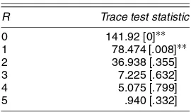
The forecasting performance of the STECM is similar to that of the STM; it will take longer to judge the effectiveness of the convergence mechanism. The VAR does not perform well on the whole. It does particularly badly for RM and does not deal well with the temporary divergence in FW. The balanced-growth VECM fares better; however, it is not as good as the STECM for two regions and is about the same for three regions. Some researchers (e.g., Carlino and Sill 2001) have been tempted to use co-integration tests to find the number of com-mon trends in U.S. regions. For our sample of six regions, the Johansen trace test, reported in Table 3, cannot reject the null hypothesis of two co-integrating vectors, that is, four common trends. However, in our view there is little point in estimating a model with two co-integrating vectors. The application of the test again simply confirms that it is misleading if series are in the process of converging.
4. COMMON AND SIMILAR CYCLES
Fitting a multivariate STM to the eight U.S. regions, as was done by Carvalho and Harvey (2005), provides a good illus-tration of the stylized facts produced by a similar (first-order) cycle model, (3), and yields an interesting comparison with the Beveridge–Nelson cycles reported by Carlino and Sill (2001). ML estimation gives a damping factor of .80 and a period of 5.3 years. In a plot of the smoothed cyclical components, the recessions of 1954, 1961, 1970, 1975, 1980, 1982, and 1991 all show up with a high degree of coherence across regions; this is not the case for the cycles estimated by Carlino and Sill (2001). There are considerable differences in volatility, with the vari-ance of the disturbvari-ances in PL being almost six times as great as that of ME. Because the expected value ofψt2+ψt∗2is 2σψ2, the amplitude of a cycle is best measured by its standard devi-ation times √2; these figures, multiplied by 100, are given in Table 4. Carlino and Sill (2001, p. 452) also reported big dif-ferences in volatility, but our ordering differs from theirs. In particular, we find that the richest regions (NE, ME, and FW) are those with the least volatile cyclical components.
Table 3. Trace Test for Co-Integration in U.S. Regions
NOTE: Computed using PcGive (see Doornik and Hendry 2001).
Table 4. Estimated Amplitudes of Cycles in Real per Capita GDP in U.S. Regions
NE ME GL PL SE SW RM FW
.9 .6 1.1 1.4 1.0 .9 1.3 .8
The extent to which similar cycles move together depends on the correlations between the disturbances driving them be-cause ψ, the covariance matrix of the vector of cycles, is (1−ρ2)−1κ. There are high positive correlations between the
cyclical disturbances in all pairs of U.S. regions. The minimum is .720, and the maximum is .987. The first principal compo-nent ofκ accounts for 91% of the total variance, whereas the
second accounts for another 5%.
4.1 Common Cycles
Ifψ is less than full rank, then there are common cycles.
If the rank ofψ is 1, there is a single common cycle, and the
model can be written as
yit=µit+θiψt+εit, i=1, . . . ,N,t=1, . . . ,T, (15)
whereψt is a scalar cycle and theθi’s allow the common
cy-cle to appear in each series with a different amplitude. One of theθi’s is set equal to unity for identifiability, and, because
the cycles have mean 0, there is no need to add a vector of constants as with common trends. A single common cycle is a common feature in the sense of Engle and Kozicki (1993) in that it may be removed by a linear combination, θ, of the observations with the property that θ′θ=0, where theN×1 vectorθ=(θ1, . . . , θN)′. [There is a slight difference between
the common cycle definition of Vahid and Engle (1993) and the foregoing in that if the series areI(1)and not co-integrated, then the former requires that there exist linear combinations whose first differences are unpredictable from their past. In a structural model with random-walk trends, the presence of an irregular component means that although a common cycle is removed byθ′yt,θ′yt has a first-order moving average representation and so is predictable. We are grateful to a referee for pointing this out.]
The common cycle constraint is a strong one, particularly if the irregular component is relatively small. Harvey and Trimbur (2003) found that fitting higher-order cycles tends to cause the irregular component to become relatively more important while the extracted cycle is smoother. Thus higher-order cycles may be better for modeling common cycles.
4.2 Testing for Common Cycles
We now consider how to test the null hypothesis of a single common cycle in a bivariate STM against the alternative of sim-ilar cycles. Under the alternative hypothesis,κis of full rank,
whereas under the null hypothesis, the correlation between the disturbances in the two cycles is 1. Because a correlation of 1 is on a boundary of the admissible parameter space, the asymp-totic distribution of the likelihood ratio (LR) statistic is an even mixture ofχ02andχ12, and the 10%,5%, and 1% critical values are 1.642, 2.706, and 5.412. This is an example of the appli-cation of a classic result of Chernoff (1954). Andrews (2001,
pp. 712–714) provided a recent unified discussion of the rel-evant theory under very general conditions. Another way of viewing this result is to transform the vector(ψ1t, ψ2t)′so that
there is a common cycle in each series and a specific cycle in one; we can then test the null hypothesis that the variance of the specific cycle is 0.
To investigate small-sample properties, we carried out a se-ries of Monte Carlo experiments on a simple bivariate cycle plus irregular model,
Only first-order and second-order cycles were considered with ρ=.9 forn=1 and .75 forn=2. The test is of the null hypoth-esis of a common cycle, that is,ω=1 against the alternative of similar cycles,ω <1. All of the results reported here are based on 10,000 replications with random numbers generated by Ox subroutines.
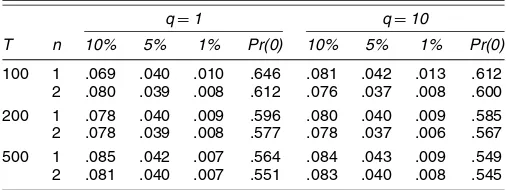
Table 5 gives the estimated test sizes for T =100,200, and 500 for signal-to-noise ratios, q=σψ2/σε2, of 1 and 10. As can be seen, there is a slight tendency for the tests to be undersized, but there is a movement toward the nominal size asTincreases. Some experiments were also run forq=.1, and these showed the test to be somewhat oversized, particularly forn=1. However, such a smallqis unlikely to arise in prac-tice. The probabilities that the LR statistic is 0 are somewhat greater than the .5 predicted by asymptotic theory, but fall as T increases and seem to be closer to .5 for higher values ofq. There is a slight tendency for the probabilities to be closer to .5 forn=2, but there is no corresponding movement in the size up toward the nominal.
Table 6 gives estimated probabilities of rejection when as-ymptotic critical values are used. Size-corrected powers would be somewhat larger for small samples. As might be anticipated, the power of the test increases withq. There appears to be little difference between first-order and second-order cycles.
For N >2, the distributional theory for the LR statistic becomes more complex, and it may be necessary to resort to simulation methods to obtain critical values (see Andrews 2001; Robin and Smith 2000; Stoel, Garre, Dolan, and van den Wittenboer 2006). For example, whenN=3,Stoel et al. (2006) showed that the asymptotic distribution of the LR statistic for a test of the null hypothesis of one common cycle against the
Table 5. Estimated Sizes of Tests Based on Asymptotic Critical Values and Probability That the Test Statistic Is Zero
q=1 q=10
Carvalho, Harvey, and Trimbur: Common Cycles, Common Trends, and Convergence 17
Table 6. Estimated Probability of Rejection at the (asymptotic) 5% Level of Significance for the Common Cycle Test
q=1 q=10
n T ω=.95 ω=.8 ω=.95 ω=.8
1 100 .202 .518 .869 .997 2 .193 .521 .886 1 1 200 .263 .760 .988 1 2 .242 .757 .994 1
alternative thatψ is of full rank is a mixture of chi-squared
with 0, 1, 2, and 3 degrees of freedom, with weights depending on the data.
4.3 Examples
This section illustrates the common cycles test with two ap-plications that have appeared in the common features literature. U.S. and Canada. Engle and Kozicki (1993) entertained the possibility of common business cycle features in U.S. and Canadian GDP. Here we investigate whether STMs with gen-eralized cyclical specifications support the notion of a common cycle. The data are the logarithms of quarterly, seasonally ad-justed real GDP from 1961:1 to 2001:4 for the United States (Source: Bureau of Economic Analysis, U.S. Department of Commerce) and Canada (Source: Statistics Canada).
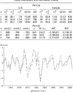
Models of the form (1), with smooth trends, were estimated with generalized cycles of order 1–6. To save space, only the results for cycles of orders 1, 2, and 4 are reported in Table 7. The first-order and second-order models show the best diagnos-tics. The second-order model would be chosen on the basis of goodness of fit as measured by the standard error of each equa-tion. The estimated period is around 7.5 years. Figures 3 and 4 show the first-order and second-order cycles obtained by state-space signal extraction. The second-order cycles are smoother. The cycles appear to differ somewhat in their timing, although on the whole the differences are slight, and there is no firm evi-dence to suggest that the U.S. cycle leads the Canadian one.
The estimated periods for the common cycle models are close to those for the similar cycle case, and the Box–Ljung Q-statistics are not very different; see Table 8. The best fit is again obtained for the second-order cycle. The load factor for Canada is .85 (the model is normalized by setting the U.S. co-efficient inθ to unity), and so the amplitude of the Canadian cycle is, on average, only .85 of that of the U.S. Figure 5 shows the extracted cycles.
The correlation between the cycle disturbances is around .8 in the similar cycle models, with the maximum being .85 for n=2. In all cases, the null hypothesis of a common cycle is convincingly rejected by the LR test. Such evidence as there
Table 7. Similar Cycle Model Fitted to U.S. and Canadian GDP: (a) Estimated Variance Parameters (×105), Equation Standard
Errors (×105), and Box–Ljung Statistics; (b) Correlations, Cycle Parameters, and Information Criteria
Part (a)
U.S. Canada
n σζ2 σψ2 σε2 Q(12) SE σζ2 σψ2 σε2 Q(12) SE
1 .08 28.1 .78 15.48 805 .13 25.8 1.04 13.13 834 2 .04 43.9 1.54 12.97 789 .09 37.5 1.83 15.78 816 4 .11 25.7 1.59 18.82 823 .14 23.6 1.81 20.49 845
Part (b)
n corr(ζ) corr(κ) corr(ε) ρ 2π/λc AIC BIC
1 .869 .796 −.763 .941 24.21 −2,185.81 −2,139.31 2 .801 .855 −.137 .794 30.5 −2,186.89 −2,140.39 4 .704 .824 −.088 .505 31.75 −2,174.94 −2,128.45
Figure 3. Similar First-Order Cycles in the U.S. ( ) and Cana-dian ( ) GDPs.
Figure 4. Similar Second-Order Cycles for the U.S. ( ) and Canadian ( ).
Table 8. Common Cycle Model for U.S. and Canadian GDP: Equation Standard Errors (×105), Goodness of Fit, Cycle Parameter Estimates, Information Criteria, and Common Cycle LR Test Statistic
U.S. Canada Cycle parameters
Test LR
Information criteria
n SE Q(12) SE Q(12) ρ 2π/λc θ AIC BIC
1 813 13.90 854 14.92 .941 21.99 .805 14.94 −2,172.86 −2,129.46 2 806 12.61 837 16.41 .767 28.80 .851 11.81 −2,177.08 −2,133.68 4 822 15.06 838 20.19 .506 28.57 .814 6.10 −2,170.85 −2,127.45
Figure 5. Common Second-Order Cycle for the U.S. ( ) and Canada ( ).
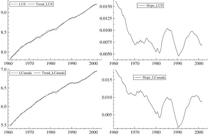
is in favor of a common cycle is strongest forn=4,but even here the LR statistic of 6.10 is well in excess of the 1% criti-cal value of 5.41. The Akaike information criterion (AIC) and Bayes information criterion (BIC) point to similar conclusions. Are U.S. and Canadian GDP co-integrated? The Johansen trace test suggests not. The probability value of a test of no cointegration (against one co-integrating vector) is .383. The STM—which hasI(2)trends—has a correlation between growth rates of .801 for n=2. The two trends are shown in Figure 6, and a simple plot of their difference makes it clear why tests reject the null. The lack of balanced growth may be due to a number of factors, for example, not using per capita data or converting currencies at an inappropriate exchange rate. Perhaps more interesting is the graph of the smoothed esti-mates of the growth rates shown in Figure 6. Both exhibit a steady decline from the 1960s coupled with long swings in the 1980s and 1990s. As with the extracted cycles, we have a near common feature.
U.S. Regions. Attempting to estimate a model for all eight U.S. regions with one common cycle led to implausible results,
even though, as noted earlier, the first principal component ac-counted for more than 90% of the total variance. The same exer-cise for quarterly data from 1969:1 to 1999:4 produced similar conclusions (see Carvalho and Harvey 2002); however, these models used only first-order cycles.
We now turn to investigating the plausibility of common cy-cles between certain pairs of U.S. regions when higher-order cycles are used. We focus on the NE and ME regions with quar-terly data where a bivariate model gives first-order cycles with a correlation of .97. Figure 7 shows the trends and cycles. As can be seen, there are slight differences in the cycles. We also note that the correlation between the slopes is .962; as with the U.S.– Canada example, it is interesting to see the extent to which the growth rates move together.
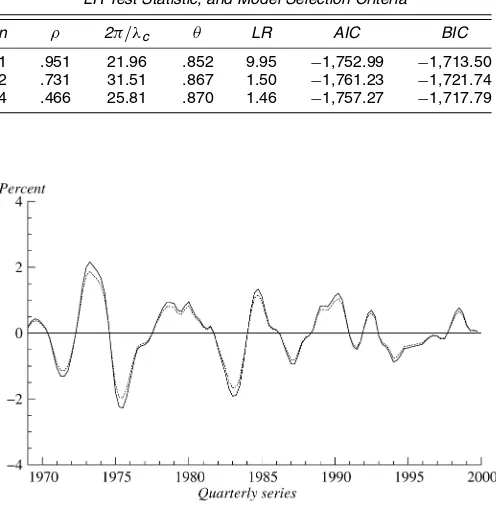
Tables 9 and 10 give the results of estimating models with higher-order cycles. The model selection criteria favor the com-mon cycle restriction forn=2 and 4, and the LR test fails to reject the null hypothesis of common cycles at the 10% level of significance in both cases, whereas forn=1 it easily rejects at the 1% level. The BIC, which for moderately large sample sizes attaches a greater penalty to model complexity, reaches a mini-mum for the second-order common cycle model. The smoothed cyclical components for the two regions are shown in Figure 8. If there is a single common cycle, then the cycles in each series in (15) have the same amplitude if θi =1 for all i=
1, . . . ,N,and so are identical. This restriction may be tested by a standard LR test in which the test statistic has aχN2
−1 distribu-tion, asymptotically, under the null hypothesis. For NE and ME, the LR test statistics forn=2 and 4 are 1.46 and 0.28, and so it seems reasonable to treat the cycles as being identical.
Although some other pairs of regions also appear to share a common higher-order cycle, there is insufficient communal-ity to allow a single common cycle for all regions even when higher-order cycles are used.
Finally we note that Vahid and Engle (1993, pp. 355–358) analyzed the four industrial regions NE, ME, GL, and FW and found three common trends, as did Carvalho and Harvey
Figure 6. Trends and Growth Rates for the U.S. and Canadian GDPs.
Carvalho, Harvey, and Trimbur: Common Cycles, Common Trends, and Convergence 19
Figure 7. Trends, Growth Rates, and (first-order) Cycles in the NE and ME U.S. Regions.
Table 9. Similar Cycle Model for per Capita GDP in NE and ME: Correlations, Cycle Parameters, and Model Selection Criteria
n corr(ζ) corr(κ) corr(ε) ρ 2π/λc AIC BIC
1 .962 .970 .797 .940 29.24 −1,760.94 −1,718.63 2 .948 .975 .829 .729 35.03 −1,760.72 −1,718.42 4 .937 .986 .828 .377 28.70 −1,756.74 −1,714.43
Table 10. Common Cycle Model for NE and ME: Cycle Parameters, LR Test Statistic, and Model Selection Criteria
n ρ 2π/λc θ LR AIC BIC
1 .951 21.96 .852 9.95 −1,752.99 −1,713.50 2 .731 31.51 .867 1.50 −1,761.23 −1,721.74 4 .466 25.81 .870 1.46 −1,757.27 −1,717.79
Figure 8. Second-Order Common Cycle in Real GDP in the NE ( ) and ME ( ) Regions of the U.S.
(2005). Whereas Vahid and Engle pointed out in their foot-note 12, page 356, that they “are not convinced that cointegra-tion is necessary for convergence,” they nevertheless estimated a VECM incorporating a co-integrating vectorME−.48NE−
.45GL−.07FW, the economic interpretation of which is un-clear to us. On the basis of canonical correlations of the first differences, they found evidence for two common cycle features that are linear combinations of the first differences. As with the co-integrating vector, we are uncertain of the meaning of these combinations.
5. CONCLUSION
Common trends are undoubtedly the most important com-mon feature of economic time series. However, data on coun-tries or regions often show that they are converging, have just converged, or converged some time earlier but still have a large part of the series dependent on initial conditions. This is cer-tainly the case with per capita GDP in the U.S. regions. Such series are not co-integrated within the sample, but the fact that they are converging to a special case of a co-integrated system—namely, balanced growth—must be taken into account if coherent medium-term forecasts are to be made. This arti-cle has reviewed the unobserved components error-correction model, the STECM, proposed in Carvalho and Harvey (2005) and compared its forecasting performance in a postsample pe-riod with unrestricted VARs and balanced-growth VECMs. The way in which the second-order error correction mechanism copes with temporary divergence is particularly appealing. In the case of the U.S. regions, the STECM forecasts well and predicts the temporary divergence of FW at the beginning of the postsample period. The relatively poor forecasts obtained with an unrestricted VAR illustrates the case for taking account of convergence to balanced growth.
Structural time series models can handle common cycles within the framework of similar cycles, and the cycle model can be generalized so that when extracted, it is relatively smooth.
We develop a LR test for common cycles in a bivariate series and apply it to the series on U.S. and Canadian GDP. Although the U.S. and Canadian cycles move closely together, the hy-pothesis that they share a common cycle is decisively rejected for a range of cyclical models. However, for some pairs of U.S. regions, it seems that a common second-order cycle cannot be rejected; the example we give is that of ME and NE.
In the bivariate case, the asymptotic critical values for the common cycle test statistic are obtained from tables of theχ12 distribution by doubling the nominal significance level. More generally, it seems difficult to find a correspondingly simple test for a specific number of common cycles. It is perhaps worth noting, however, that common cycle restrictions may not offer significant gains in forecasting; making allowances for the cy-cles being highly correlated may be all that is needed.
Finally, we note that because a structural time series model can include several components, the possibility of more than two common features can be entertained. In particular, it is easy to allow for common seasonal effects, and seasonal co-integration tests can be carried out as described by Busetti (2006).
ACKNOWLEDGMENTS
The initial stages of the work on convergence was supported by the ESRC as part of a project on Dynamic Factor Models for Regional Time Series (grant L138 25 1008). Trimbur acknowl-edges the support of the U.S. Census Bureau during his time as a postdoctoral researcher. Carvalho acknowledges the financial support of the Portuguese Ministry of Science and Technology and The University of Chicago. Note that the analysis and con-clusions set forth in the article do not indicate concurrence by the Board of Governors or the staff of the Federal Reserve Sys-tem. The authors thank Bill Bell, David Findley, and Richard J. Smith, the referees and participants at the ESRC Econometric Study Group meeting at IFS, May 2005, for helpful comments. Special thanks go to Giovanni Urga for encouraging then to write the article in the first place and seeing it through various drafts.
[Received April 2005. Revised February 2006.]
REFERENCES
Andrews, D. W. K. (2001), “Testing When a Parameter Is on the Boundary of the Maintained Hypothesis,”Econometrica, 69, 683–734.
Busetti, F. (2006), “Tests of Seasonal Integration and Cointegration in Multi-variate Unobserved Component Models,”Journal of Applied Econometrics, 21, 419–438.
Carlino, G., and Sill, K. (2001), “Regional Income Fluctuations: Common Trends and Common Cycles,” Review of Economics and Statistics, 83, 446–456.
Carvalho, V. M., and Harvey, A. C. (2002), “Growth, Cycles and Convergence in U.S. Regional Time Series,” DAE Working Paper 0221, University of Cambridge.
(2005), “Growth, Cycles and Convergence in U.S. Regional Time Se-ries,”International Journal of Forecasting, 21, 667–686.
Chernoff, H. (1954), “On the Distribution of the Likelihood Ratio,”The Annals of Mathematical Statistics, 25, 573–578.
Doornik, J. A. (1999),Ox: An Object-Oriented Matrix Language(3rd ed.), Lon-don: Timberlake Consultants.
Doornik, J. A., and Hendry, D. F. (2001),Modelling Dynamic Systems Using PcGive, Vol. II, London: Timberlake Consultants.
Engle, R. F., and Kozicki, S. (1993), “Testing for Common Features,”Journal of Business & Economic Statistics, 11, 369–380.
Harvey, A. C. (1989),Forecasting, Structural Time Series Models and the Kalman Filter, Cambridge, U.K.: Cambridge University Press.
Harvey, A. C., and Koopman, S. J. (1997), “Multivariate Structural Time Se-ries Models,” inSystem Dynamics in Economic and Financial Models, eds. C. Heij, J. M. Schumacher, B. Hanzon, and C. Praagman, Chichester: Wiley, pp. 269–298.
(2000), “Signal Extraction and the Formulation of Unobserved Com-ponents Models,”Econometrics Journal, 3, 84–107.
Harvey, A. C., and Trimbur, T. (2003), “General Model-Based Filters for Ex-tracting Trends and Cycles in Economic Time Series,”Review of Economics and Statistics, 85, 244–255.
Koopman, S. J., Harvey, A. C., Doornik, J. A., and Shephard, N. (2000),
STAMP 6.0 Structural Time Series Analyser, Modeller and Predictor, Lon-don: Timberlake Consultants.
Koopman, S. J., Shephard, N., and Doornik, J. A. (1999), “Statistical Algo-rithms for Models in State-Space Form Using SsfPack 2.2” (with discussion),
Econometrics Journal, 2, 107–160.
Robin, J.-M., and Smith, R. J. (2000), “Tests of Rank,”Econometric Theory, 16, 151–175.
Rünstler, G. (2004), “Modelling Phase Shifts Among Stochastic Cycles,”
Econometrics Journal, 7, 232–248.
Stoel, R. D., Garre, F. G., Dolan, C., and van den Wittenboer, G. (2006), “On the Likelihood Ratio Test in Structural Equation Modeling When Parameters Are Subject to Boundary Constraints,”Psychological Methods, to appear. Trimbur, T. (2006), “Properties of Higher-Order Stochastic Cycles,”Journal of
Time Series Analysis, 27, 1–17.
Vahid, F., and Engle, R. F. (1993), “Common Trends and Common Cycles,”
Journal of Applied Econometrics, 8, 341–360.