New parameter relationships determined via stochastic
ordering for spike activity in a reversal potential neural
model
Laura Sacerdote
a,*, Charles E. Smith
baDepartment of Mathematics,Uni
6ersity of Torino,Via Carlo Alberto10,10123Torino,Italy
bNCSU Department of Statistics,2700Stinson Dri
6e Campus Box8203,110Cox Hall,Raleigh,NC27695-8203,USA
Abstract
Purpose of this work is to study the dependence of interspike interval distribution on the model parameters when use is made of the Feller diffusion process to describe the subthreshold membrane potential of a neuron. To this aim we make use of a new approach, namely the ordering of first passage times. The functional dependence among the model parameters (e.g. membrane time constant, reversal potential, etc.) resulting from the ordering criteria employed and from the study of mean trajectory plots is analyzed into detail for four different scenario. © 2000 Elsevier Science Ireland Ltd. All rights reserved.
Keywords:Feller model; Stochastic order; Interspike interval distribution
www.elsevier.com/locate/biosystems
1. Introduction
The Feller process has been proposed as a model of subthreshold membrane behavior by various authors (cf. Hanson and Tuckwell, 1983; La´nsky´ and La´nska´, 1987; Giorno et al., 1988; La´nska´ et al., 1994). A realistic advantage of this model with respect to the Ornstein – Uhlenbeck process is that the introduction of this particular state-dependent changes in depolarization con-strains the membrane potential values to a finite interval. No procedure exists to obtain closed
form expressions for the firing distribution, so both models have been investigated in many ways. Numerical methods have been used to study the firing times corresponding to different choices of the parameters characterizing the two models in (Ricciardi and Sacerdote, 1979; Giorno et al., 1988) while in La´nsky´ et al. (1995) interspike interval (ISI) distributions obtained from the Feller model are compared with those obtained from the Ornstein-Uhlenbeck model. However numerical methods are of little help if one is interested in determining the functional
depen-dence of ISI distribution on the model
parameters.
The features of the Ornstein-Uhlenbeck model can help the intuition if one wishes to understand
* Corresponding author.
E-mail addresses: [email protected] (L. Sacerdote), [email protected] (C.E. Smith).
the effect of a parameter value on the ISI distribu-tion. On the other hand, this approach cannot be employed in the case of the Feller model since the complexity of the underlying mathematical process limits to a few instances the use of this method. Indeed, as we illustrate in Section 2 by means of some examples, the use of mean trajectory plots is useful in understanding the dependences of the Feller model on the parameters only if spikes correspond to the so called ‘deterministic crossings’ (cf. Smith, 1992).
Here we propose a new approach to the study of the parameter dependence of ISI distributions. We make use of a theorem proved in (Sacerdote and Smith, 1999) to order first passage times (FPT) corresponding to different processes. In Section 3 we re-state this theorem in the particular instance of the comparison of first passage times for two Feller processes characterized by two different set of values of the parameters.
In Section 4 we analyze, with the help of the aforementioned theorem, the dependence of ISI intervals on the values of the inhibitory reversal potential, the membrane spontaneous decay time constant, the noise characterizing the model and the net excitation impinging upon the neuron. Furthermore we determine different sets of values for the parameters corresponding to the same ISI distribution. For example we can prove in this way that a percent change of the coefficient describing the noise of the membrane can be balanced by a corresponding percent variation of the values of the boundary, of the reversal potential and of the net excitation.
2. The model
Classical Stein’s model (cf. Stein, 1965) for the description of the membrane potential, adapted to consider inhibitory reversal potentials, is given by the stochastic differential equation (SDE) (cf. La´n-sky´ and La´nska´, 1987):
dYt=
constants and N+
={N+(
t), t]0}, N−
={N−
(t), t]0} are two independent homogeneous Pois-son processes with intensitiesl,vrespectively. The constant VIrepresents the inhibitory reversal po-tential, ais the size of the excitatory postsynaptic potential (EPSP) andocharacterizes the size of the inhibitory postsynaptic potential (IPSP).
jis a random variable, independent ofN+,N−,
defined in an appropriate interval in order to avoid a jump to values belowVI, and for whichE(j)=0. The corresponding diffusion model, known as the Feller model (cf. La´nsky´ et al., 1995), is defined by the SDE:
suitable limiting procedure performed on a se-quence of models Eq. (1) andW={W(t), t]0} is a Wiener process. The mean trajectory of the model is
E(YtY0=0)=mu(1−e
−t/u) (4)
and the variance of the trajectories is
Var(YtY0=0)
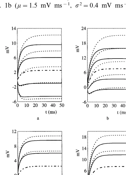
A first approach to determining the dependency of FPT on the individual parameters comes from considering mean trajectory plots, obtained by plotting (4) as a function oft and considering the
bands obtained adding 9Var(YtY0=0) or 9
2Var(YtY0=0) to its value. Fig. 1 a – d are
examples of these plots obtained by varying the parametersu, mand VI respectively.
The values used for these parameters are in a biologically reasonable range (cf. La´nsky´ et al., 1995 and references quoted therein). For the case considered in Fig. 1a (m=0.5 mV ms−1,s2=0.4
mV ms−1
, VI= −10 mV, u=5 or 7 ms
respec-tively; mean trajectories: u=7 ms dotted line,
u=5 ms dashed-dotted line; from top to bottom:
upper and lower limits for u=7 ms dashed line,
u=5 ms thick line), crossing of a boundary in
S=10 is due to the noise, while for the case of
Fig. 1b (m=1.5 mV ms−1, s2=0.4 mV ms−1,
VI= −10 mV, u=5 or 7 ms respectively; same
lines caption as before) there are deterministic
crossings when u=7 ms.
In this last instance we can easily deduce from Fig. 1b that FPT corresponding to higher values
of u are faster. However an analogous approach
cannot be used for the instances considered in Fig. 1a, since crossings are due to the noise and the shapes of the mean trajectories look quite similar.
An analogous problem arises when one at-tempts to understand the dependence of FPTs on
VI. Some authors propose a value of −10 mV (cf. La´nsky´ et al., 1995 and references quoted therein)
while others suggest VI= −7 mV, but it is not
easy to understand the implications of these two choices on firing times. Indeed, as shown by the mean trajectory plots in Fig. 1c – d, (whens2=0.4
mV ms−1, u=5 ms, V
I= −7 or −10 mV and
m=0.5 or 1.5 mV ms−1, respectively; mean
tra-jectories:VI= −7 mV coincident withVI= −10
mV dashed-dotted line; from top to bottom:
up-per and lower limits forVI= −7 ms dashed line,
VI= −10 ms thick line), for these instances the
boundary crossings are caused by the noise. Fur-thermore use of the analytical expressions (4) and (5) becomes difficult as the parameters values are changed simultaneously. Hence the use of an al-ternative approach to this analysis seems desirable to improve the understanding of this model. In the next Section we consider a new method to compare the ISI interval distributions as the parameters values change.
3. Comparison of FPTs
In many instances it looks difficult to determine closed form expressions for FPTs and hence com-paring interspike distributions seems a hard task. However, focusing on phenomena driven by the same noise values, it is obvious that when each sample path of a first process assumes values that are always larger than the corresponding ones for the second process the interspike intervals will be smaller for the first model. Furthermore in this instance the FPT distribution for the first model is
Fig. 1. Mean trajectory plots illustrating the dependence of FPT onu
dominated by the FPT distribution of the second one.
One could suppose that the same ordering be-tween FPTs is likely to arise in different in-stances, corresponding to particular choices for the parameters characterizing the models. A mathematical approach to these question has been proposed in Sacerdote and Smith (1999) where theorems useful for ordering first passage times of diffusion processes through boundaries have been proved. Making use of the
mathemati-cal tools provided in that paper we can
consider the case of two diffusions Y1, Y2
satisfying the SDE (2) driven by the same noise
process W and characterized by parameters
(u1, m1, s1, VI
1,
S, y0) and (u2, m2, s2, VI
2,
S, y0) respectively. For easy of notation from
now on we will set ak=1/sk
2(m
k−VI k/u
k), k= 1, 2 . If the parameters satisfy one of the two following relationships:
with probability one. This means that if we com-pare the interspike intervals corresponding to the models characterized by the parameters indexed 1 with the analogous ones for the model indexed 2, always considering processes characterized by
the same driving noise W, we are sure that the
last ones are always larger than the others. Fur-thermore inequality Eq. (8) holds if
c.
!
u1]u2 a1Ba2(9)
and the lower process is constrained by a reflect-ing boundary in
We can use relationships (6), (7) and (9) to study the effect of changes in the parameters values on the model features. In particular we can compare the distributions of interspike inter-vals since, as we have already mentioned, when the values corresponding to the same driving noise are ordered it follows that the distributions are ordered (cf. Shaked and Shanthikumar, 1988). Hence by means of (6), (7) and (9) we can determine ranges of parameters values that in-crease the interspike intervals.
Note that condition (10) adds a new hypothe-sis to the model by introducing a boundary that cannot be justified from a biological point of view. However, as we will see in the next Section by means of some numerical examples, inequality (8) holds under more general instances and the interspike intervals comparison can be used to understand the role of the parameters when they vary in a larger range. Furthermore, when the parameters are in a biologically interesting range, condition (10) can be removed without introduc-ing serious errors and the validity of the
relation-ship (8) is kept for the models under
consideration.
Another approach to the analysis of the parameters dependence of interspike interval dis-tributions consists in determining possible differ-ent values for the parameters of the same model that produce equal first passage times. The ratio-nal for this study is strictly related to the prob-lem of estimating the parameters values from samples of interspike intervals. In order to un-derstand if it is possible that two different
pro-cesses give rise to the same interspike
gi(y)=
It is a simple matter of calculus to observe that if
(a) u1=u2
Hence we are able to determine sets of parame-ters values for two different processes that lead to the same interspike distribution.
4. Results and discussion
We consider here some particular choices of parameters values for which (6) and (7) or (9) hold. If we do not explicitly state different values for the boundary and the initial value, we always
assume S=10 mV,y0=0 mV.
As a first scenario we analyze the dependence of
interspike intervals on u which is function of the
membrane time constant t and of the IPSPs via
(3). Consider two models characterized by equal values for all the parameters except that u1\u2.
In this case condition (9) is verified. Hence first passage times are inversely proportional to the
value ofufor a model with a reflecting boundary
aty. However, if the absorbing boundarySis far
enough from VI the presence of the reflecting
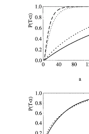
boundary (10) does not effect the order relation-ships between FPTs and can be disregarded. Hence (8) holds for the original model. In Fig. 2a we give an example of some instances where (8) holds. We plot the first passage time distribution
for u=5,7 ms, m=0,1 mV ms−1, s2
=0.4 mV
ms−1 and V
I= −10 mV. Fig. 2b exemplifies a
case where the effect of (10) cannot be disre-garded. Indeed high depolarization values of the
Fig. 2. FPT distributions ((a) from top to bottom:u=7 ms,
m=1 mV ms−1;u=5 ms,m=1 mV ms−1;u=7 ms,m=0
mV ms−1;u=5 ms,m=0 mV ms−1; (b)u=3.5 ms,
continu-ous line, andu=8 ms, dashed line).
membrane potential become attainable because of
the smaller value of VI= −7 mV and of the
larger noise coefficient s2=1.6 mV ms−1. In this
instance the spikes times are not ordered, for
example if u=3.5 and 8 ms as shown in Fig. 2b.
The second scenario considers the effect of decreasing the value ofVI. Making use of (6) with all the parameters equal in the two models except
VI
(1)B VI
(2)
, the FPT for the first model is smaller than for the second. Note that this result cannot be easily explained by resorting to intuition. In-deed we have smaller firing times when we con-sider a larger diffusion interval for the membrane potential process. However we emphasizes that the role ofVIis more complex since it changes the effect of IPSPs on the membrane potential behav-ior. In Fig. 3 we illustrate by means of two different examples the theoretical results
concern-ing the role of VI obtained from (6). The two
curves on the top compare the FPT distributions
of two models characterized byVI= −10 or −7
mV, m=1 mV ms−1
, s2
=0.4 mV ms−1
Fig. 3. FPT distributions. From top to bottomVI= −10 mV,
m=1 mV ms−1; V
I= −7 mV, m=1 mV ms−1; VI= −10
mV,m=0 mV ms−1;V
I= −7 mV,m=1 mV ms−1.
Fig. 5. Different choices for the parameters give rise to the same FPT probability density (a) and distribution (b).
the same choices of values except that m=0 mV
ms−1. Note that for both sets of parameters the
FPT can be ordered but when one introduces a net positive excitation the distance between the two curves decreases. Hence in this instance the model is less effected by the values of the rever-sal potential.
The next situation considers the dependence
of the ISI distribution on m. Use of (6) in this
instance confirms our intuition. Indeed a larger net excitation implies smaller ISIs if the other parameters are kept equal. Fig. 4 illustrates this
result when u=5 ms, s2=0.4 mV ms−1, V
I=
−10 mV and m= −0.5, 0, 0.5, 1 mV ms−1,
respectively.
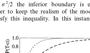
Afterwards we consider the dependence of
FPT on the noise parameter s2. Since, following
Feller’s classification of boundaries, for m−VI/
u]s2/2 the inferior boundary is entrance, in
order to keep the realism of the model s2
must satisfy this inequality. In this instance, if s1
2B
s2
2, the FPT of the first model is faster than the
corresponding value for the second one. This confirms the intuition that noise facilitates the crossings.
In these four scenarios we have tried to un-derstand the effect of changing an individual parameter. However our ordering results can be used in more complex circumstances when more than one parameter vary and the intuition from the simple inspection of mean trajectories can lead to misleading results.
Finally we analyze an application of (12). We consider the following instance: assume we have determined the value of the infinitesimal vari-ance with a possible error of 10%. We want to understand whether this error can be balanced by a variation in the values of the other parameters to obtain equal FPTs. Making use of condition (12) it is easy to see that if,
corre-sponding to an increased value of s2 we
in-crease by the same percentage the coefficient m
the boundary value and decrease the reversal potential, the FPT distribu-tion cannot change. The curve in Fig. 5 can be drawn either with
the choice for the parameters s2
=0.4 mV, u=
0.5 ms, m=1 mV ms−1
, VI= −10 mV, S=10
mV and y0=0 mV or with the choice s
2 =5
mV, u=5 ms, m=1 mV ms−1,
VI= −11 mV,
S=11 mV and y0=0 mV. In the same way we
could determine many other instances that give rise to the same shape. Hence we cannot uniquely determine parameters values just from measures of ISIs.
5. Conclusions
In this work different approaches have been considered in order to understand the dependence of interspike interval distribution on the parame-ters characterizing the phenomena when one con-sider a neuronal model with reversal potential. We have shown that in some instances a simple intu-itive approach via trajectory plots can give rise to misleading results. Hence here we have proposed to use the ordering criteria introduced in Sacerdote and Smith (1999) to investigate the role of the parameters in the model. We explicitly remark that the validity of this method is not restricted to the case considered, but could be extended to the comparison of different neuronal diffusion models proposed in literature. This will be the content of a forthcoming paper where we plan to analyze the model with inhibitory and excitatory reversal po-tentials proposed in La´nska´ et al. (1994).
Acknowledgements
The work for this paper was done when the first named author was visiting NCSU at Raleigh, NC. She would like to thank her colleagues at the Department of Statistics for their kind hospitality. Work supported by C.N.R. contract 98.01033. CT01 and by INDAM.
References
Giorno, V., La´nsky´, P., Nobile, A.G., Ricciardi, L.M., 1988. Diffusion approximation and first-passage-time problem for a model neuron. III. A birth-and-death approach. Biol. Cybern. 58, 387 – 404.
Hanson, F.B., Tuckwell, H.C., 1983. Diffusion approxima-tion for neuronal activity including synaptic reversal po-tentials. J. Theor. Neurobiol. 2, 127 – 153.
La´nsky´, P., La´nska´, V., 1987. Diffusion approximations of the neuronal model with synaptic reversal potentials. Biol. Cybern. 56, 19 – 26.
La´nsky´, P., Sacerdote, L., Tomassetti, F., 1995. On the com-parison of Feller and Ornstein-Uhlenbeck models for neural activity. Biol. Cybern. 73, 457 – 465.
La´nska´, V., La´nsky´, P., Smith, C.E., 1994. Synaptic trans-mission in a diffusion model for neural activity. J. Theor. Biol. 166, 393 – 406.
Ricciardi, L.M., Sacerdote, L., 1979. The Ornstein-Uhlen-beck process as a model for neuronal activity. Biol. Cy-bern. 35, 1 – 9.
Sacerdote, L. Smith, C.E. 1999. Stochastic ordering for first passage times of diffusion processes through boundaries. Mimeo Series 2515, Institute of Statistics, North Caro-lina State University, Raleigh, NC, USA.
Shaked, M., Shanthikumar, J.G., 1988. On the 1st passage times of pure jump-processes. J. Appl. Prob. 20 (2), 427 – 446.
Smith, C.E., 1992. A heuristic approach to stochastic models of single neurons. In: Neural Nets: Foundations and Ap-plications. Academic Press, New York, pp. 561 – 587. Stein, R.B., 1965. A theoretical analysis of neuronal
variabil-ity. Biophys. J. 5, 173 – 195.