*Corresponding author. Tel.:#49-521-106-3929; fax:# 49-521-106-6036.
E-mail address:[email protected] (D. Biskup).
A note on
&
An e
$
cient algorithm for the single-machine
tardiness problem
'
Dirk Biskup*, Wolfgang Piewitt
Faculty of Economics and Business Administration, University of Bielefeld, Postfach 10 01 31, 33501 Bielefeld, Germany Received 20 April 1998; accepted 20 December 1999
Abstract
The focus of this work is to give some comments on a paper recently published by Kondakci et al. (International Journal of Production Economics 36 (1994) 213}219). They present a new branch-and-bound algorithm for the famous total tardiness problem. However, some aspects of the algorithm remain vague, namely the application of the labelling scheme of Schrage and Baker (Operations Research 26 (1978) 444}449), the calculation of the lower bounds and the utilisation of Elmaghraby's (Journal of Industrial Engineering 19 (1968) 105}108) dominance theorem. As limiting total enumeration is the most interesting part of a branch-and-bound algorithm we clarify the inaccuracies and propose a fast recursion to calculate the lower bounds. We demonstrate the branch-and-bound algorithm by using an example. ( 2000 Elsevier Science B.V. All rights reserved.
Keywords: Scheduling; Single machine; Tardiness; Branch-and-bound
1. Introduction
The total tardiness problem (TTP) is one of the most famous problems in single-machine schedul-ing theory. It has been receivschedul-ing considerable atten-tion since the excellent paper of Smith [1]. Recently, the TTP has been proven to be NP-hard [2]. Kondakci et al. [3] present an interesting branch-and-bound algorithm for the TTP. How-ever, some aspects of their algorithm remain impen-etrable. The focus of this note is to clarify those. Furthermore, we present a fast recursion to calcu-late the lower bounds.
2. Problem de5nition and bounds
Using the notation of Kondakci et al. [3] there arenjobs available at a time zero with processing times p
i and distinct due dates di for all jobs
i"1,2,n. They have to be processed on a con-tinuously available machine, pre-emption is not allowed. CT
i and ¹i"maxM0, CTi!diN denote the completion time and tardiness of job i,
i"1,2,n, respectively. The objective is to "nd a schedule minimising+ni/1¹
i.
Kondakci et al. [3] obtain a lower bound for the problem by solving the so-called generalised prob-lem, wherenjobs with processing times andndue dates are given. Contrary to the TTP the due dates are not linked together with the jobs, therefore they can be assigned to the jobs arbitrarily. The ob-jective function value of the generalised TTP is
minimised by scheduling the jobs according to the shortest processing time (SPT) rule and assigning the smallest due date to the "rst job, the second smallest due date to the second job, etc. (see [4]).
An initial upper bound is obtained by applying priority rules, Emmons'theorems (see Appendix A) and a modi"ed version of Moore's algorithm to the TTP and selecting the sequence with the lowest objective function value.
3. The branch-and-bound algorithm
Generally, a schedule is constructed backwards. Let a partial schedule be a set of jobsJ
S which are
assigned to the last positions and are sequenced in a distinct manner. Further, letJ
U"M1, 2,2,nNCJS
be the set of unscheduled jobs. Each node at the level t of the tree represents a partial schedule ([n!t#1], [n!t#2],2, [n]), where [k] de-notes the job assigned to the kth position of the schedule. At the leveltof the tree the branching is done by optionally assigning each of then!t un-scheduled jobs to the (n!t)th position of the schedule. Hence, for each parent node at the level
tthere aren!tdescendent nodes.
The labelling of the nodes could be done by applying the labelling scheme of Schrage and Baker [5] (see Appendix A) to the corresponding partial schedule. This seems advantageous for two reasons: Firstly, nodes with the same label must contain the same set of jobs (in a di!erent order). Hence, if there are two or more nodes with the same label only the node with the smallest lower bound needs to be regarded for branching; the other nodes can be fathomed, because they cannot lead to a superior schedule. Secondly, when applying the dominance theorem of Elmaghraby [6] mentioned further down it is easy to"nd the node representing a par-tial schedule to be used in dominance tests. If com-paring two partial schedules J
1 and J2, with J
1-J2, let J$*&"J2CJ1 be the set of jobs solely
belonging to the partial scheduleJ
2. Then the label
of the node representingJ
1equals the label of the
node representingJ
2minus the sum of the labelling
numbers of the jobs inJ
$*&.
The lower bound of a node could be obtained as follows: For the jobs assigned to the partial
sched-ule, that is for the jobs inJ
S, the total tardiness is
calculated. For the set of unscheduled jobs, J U,
a generalised problem is solved. Letf
'be the
objec-tive function value of the generalised problem. Thus the lower bound of a node is gained by adding up the total tardiness of the partial schedule andf
'.
A fast method to calculate this lower bound, especially the total tardiness of the partial schedule is given by the following recursion: Let¸
JS be the label of the node representing a partial schedule consisting of the jobsJ
S. Note, that this relation is
a consequence of the application of the labelling scheme of Schrage and Baker [5]. Usually the tardiness of the partial schedule at the node
¸ Alternatively, ¹(¸
JS) can be calculated by recur-sion, because the tardiness of all jobs but the"rst have been determined at the parent node of ¸
JS.
with jobjoccupying the"rst position of the partial schedule. Further, let¸
k be the labelling numbers of the jobsk,k"1,2,n. Now the lower bound of a node can easily be calculated by
¸B(¸
Elmaghraby's dominance tests are applied to par-tial schedules that di!er by one job at the most. Unfortunately, the presentation of the theorem contains a#aw by Kondakci et al. [3]. The correct version is: If two partial schedulesJ
with J
1-J2 and ¹(J1)*¹(J2) then the partial
scheduleJ
2 dominatesJ1 and the node
represent-ingJ
1 can be fathomed. In combination with the
labelling scheme of Schrage and Baker [5] the following Lemma 1 can be stated.
Lemma 1. Given two partial schedulesJ
1andJ2the following holds: J
1 dominates J2 if ¸J1"¸J2 or
Proof. Trivial from the argumentation above. h
It is well-known that the size of an instance can often be reduced by applying Emmons'Theorems. Therefore, only reduced problems are considered. Nevertheless, the branch-and-bound algorithm can be improved by using the results of Emmons' the-orems, because it is usually possible to identify some precedence relationships between the remain-ing jobs. These relationships will be stored in a so-called precedence matrix, see [7] and used to reduce the branching. Thus a job can only be assigned to a node if all its successors are already included inJ
S. For example, at the"rst level of the
tree only jobs without any successors are regarded as candidates.
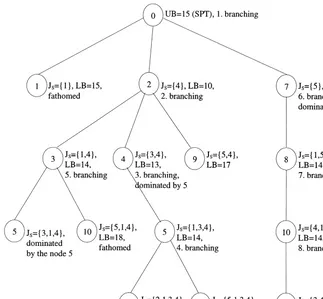
The branch-and-bound algorithm is demon-strated on the following Example 1, rather than the example used by Kondakci et al. [3] as this can be solved completely by applying Emmons' theorems.
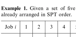
Example 1. Given a set of "ve jobs, which are already arranged in SPT order.
Jobi 1 2 3 4 5
p
i 1 2 3 4 6
d
i 10 7 7 8 3
The initial upper bound of 15 is obtained from the SPT order of the jobs. By applying Emmons' the-orems, the following precedence constraints matrix
is received:
According to the labelling scheme of Schrage and Baker [5], the labelling numbers of the jobs are
¸
1"1,¸2"1,¸3"2,¸4"2 and¸5"7. Note
that even if two jobs have the same labelling num-ber there cannot exist two or more nodes with equal labels representing distinct partial schedules. Because of the precedence constraints, for example, neither job 2 nor job 3 could be at the last position in an optimal schedule. Therefore, at the"rst level of the tree, only the jobs 1, 4 and 5 are considered as a partial schedule (see Fig. 1).
Table 1 demonstrates the procedure of the branch-and-bound algorithm of Example 1. The values in the"fth column¹(¸
JS) represent the tar-diness costs which are incurred at the node¸
JS by the partial schedule J
S. They are obtained by the
recursion (*) as a result of the sum of the tardiness costs of the parent node, ¹(¸
JS!¸j), and the tardiness of the last job assigned to the node,
¹
j"maxM0,+i|JUpi#pj!djN. In the sixth column, the nodes which are considered by the dominance tests are listed: At the left-hand side of the diagonal stroke the candidate nodes are re-corded, which could dominate the node ¸
JS. To these nodes the "rst part of Lemma 1 is applied. On the right-hand side the candidate nodes which could be dominated by¸
JS are listed. To them the second part of Lemma 1 is applied. The seventh column states the objective function of the generalized problem for the unscheduled jobsJ
U,
which added to¹(¸
JS) gives the lower bound of the node, that is LB(J
S). The last column contains some
Fig. 1. The branch-and-bound tree of Example 1.
The branch-and-bound algorithm is illustrated at the tree in Fig. 1.
4. Conclusions
With this paper we clarify some aspects of the branch-and-bound algorithm for the TTP present-ed by Kondakci et al. [3]. Furthermore, we suggest some re"nements to the quality of the algorithm. For the sake of demonstration an example is given.
Appendix A
A.1. Emmons'theorems
Assume thenjobs are ordered according to the SPT-rule; that is i(j if p
i(pj or pi"pj and
d
i)dj. Further let Bi be the set of jobs that are processed prior to the jobiin an optimal schedule and similarlyA
i the set of jobs that are succeeding job i in an optimal sequence. There are three theorems altogether:
Theorem 1. If
i(j and d
i)max
G
dj,pj#+ k|Bjp
k
H
then job i is produced prior to job j in an optimal schedule(i3B
j andj3Ai).
Theorem 2. If
i(j, d
i'max
G
dj,pj#+ k|Bjp
k
H
andd
i#pi*+ k|Aj
p
Table 1
The branch and bound algorithm demonstrated by Example 1
J
S ¸JS ¹(¸JS!¸j) ¹j ¹(¸JS) Lemma 1
applied to
f
' ¸B(JS) Remarks
H 0 } } 0 } } } 1. branching
1 1 0 6 6 }/} 9 15 canceled
4 2 0 8 8 }/} 2 10 2. branching
5 7 0 13 13 }/} 0 13 6. branching/
dom. by 8
1, 4 3 8 2 10 1, 2/} 4 14 5. branching
3, 4 4 8 5 13 2/} 0 13 3. branching/
dom. by 5
5, 4 9 8 9 17 2, 7/} 0 17 canceled
1, 3, 4 5 13 0 13 3, 4/} 1 14 4. branching
2, 1, 3, 4 6 13 1 14 5/} 3 17 canceled
5, 1, 3, 4 12 13 5 18 5/} 0 18 canceled
3, 1, 4 5 10 4 14 3, 5/5 } } dom. by 5
5, 1, 4 10 10 8 18 3/} 0 18 canceled
1, 5 8 13 0 13 7/} 1 14 7. branching
4, 1, 5 10 13 1 14 }/} 0 14 8. branching
3, 4, 1, 5 12 14 0 14 }/} 0 14 opt. solution
where AMj"MiDiNA
jN,then job i is produced after job
j in an optimal schedule(i3A
j and j3Bi).
Theorem 3. If i(j and d
j*+k|Ajpk, then job i is produced prior to job j in an optimal schedule.
The proofs for the three theorems are given by Emmons [8]; further information about the ap-plication of Emmon's theorems and some more literature on this topic can be found in [9]. Note that the application of Emmon's theorems to a special instance of the TTP results in a precedence constraints matrix as given above; for Example 1
A
2"M1, 3, 4NorB4"M2, 3N.
A.2. The labelling scheme of Schrage and Baker
By the labelling scheme of Schrage and Baker each single job gets a label; the label of a jobi is denoted by¸(i). The label of a set of jobsJ
S,¸(JS),
equals the sum of the labels of the jobs inJ
S; hence,
¸(J
S!MiN)"¸(JS)!¸(i). Assume the jobs are
in-dexed so that ifiis a predecessor ofjtheni(j. Let
b(j) be the sum of the labels of all jobsi(jwith
i3B
j and a(j) be the sum of the labels of all jobs
i(jwithi3A
j, respectively. Further lett(j) be the sum of the labels of all jobsi(j. Now the labelling of the jobs is done by the following algorithm: Step 1: t(i)"a(i)"b(i)"0 for i"1,2,n. Step 2: i"1.
Step 3: ¸(i)"t(i)!a(i)!b(i)#1. If i"n then stop.
Step 4: Fork"i#1, i#2,2,ndo: (a) Ifk3A
i thenb(k)"b(k)#¸(i). (b) Ifk3B
i thena(k)"a(k)#¸(i). Step 5: t(i#1)"t(i)#¸(i).i"i#1. Go to Step
3.
References
[1] W.E. Smith, Various optimizers for single-stage pro-duction, Naval Research Logistics Quarterly 3 (1956) 59}66.
[2] J. Du, J.Y.-T. Leung, Minimizing total tardiness on one machine is NP-hard, Mathematics of Operations Research 15 (1990) 483}495.
[3] S. Kondakci, OG. Kirca, M. Azizoglu, An e$cient algo-rithm for the single machine tardiness problem, Inter-national Journal of Production Economics 36 (1994) 213}219.
[4] N.G. Hall, Scheduling problems with generalized due dates, IIE Transactions 18 (1986) 220}222.
[5] L. Schrage, K.R. Baker, Dynamic programming solution of sequencing problems with precedence constraints, Opera-tions Research 26 (1978) 444}449.
[6] S.E. Elmaghraby, The one machine sequencing problem with delay costs, Journal of Industrial Engineering 19 (1968) 105}108.
[7] V. Srinivasan, A hybrid algorithm for the one machine sequencing problem to minimize total tardiness, Naval Re-search Logistics Quarterly 18 (1971) 317}327.
[8] H. Emmons, One-machine sequencing to minimize certain functions of job tardiness, Operations Research 17 (1969) 701}715.