SUPERVISED AND UNSUPERVISED MRF BASED 3D SCENE CLASSIFICATION IN
MULTIPLE VIEW AIRBORNE OBLIQUE IMAGES
M. Gerkeaand J. Xiaob
a
University of Twente, Faculty of Geo-Information Science and Earth Observation – ITC, Department of Earth Observation Science, Hengelosestraat 99, P.O. Box 217, 7500AE Enschede, The Netherlands – [email protected]
b
Computer School of Wuhan University, Luoyu Lu 129, Wuhan, P.R. China, 430072 – [email protected]
KEY WORDS:Classification, Graph Cut, Learning, Performance, Point Cloud, Optimization, Random Trees
ABSTRACT:
In this paper we develop and compare two methods for scene classification in 3D object space, that is, not single image pixels get classified, but voxels which carry geometric, textural and color information collected from the airborne oblique images and derived products like point clouds from dense image matching. One method is supervised, i.e. relies on training data provided by an operator. We use Random Trees for the actual training and prediction tasks. The second method is unsupervised, thus does not ask for any user interaction. We formulate this classification task as a Markov-Random-Field problem and employ graph cuts for the actual optimization procedure.
Two test areas are used to test and evaluate both techniques. In the Haiti dataset we are confronted with largely destroyed built-up areas since the images were taken after the earthquake in January 2010, while in the second case we use images taken over Enschede, a typical Central European city. For the Haiti case it is difficult to provide clear class definitions, and this is also reflected in the overall classification accuracy; it is 73% for the supervised and only 59% for the unsupervised method. If classes are defined more unambiguously like in the Enschede area, results are much better (85% vs. 78%). In conclusion the results are acceptable, also taking into account that the point cloud used for geometric features is not of good quality and no infrared channel is available to support vegetation classification.
1 INTRODUCTION AND RELATED WORK
Oblique airborne imaging is entering more and more into pho-togrammetric production workflows. For a relatively long time Pictometry and the Midas Track’Air system have been a stan-dard in small format multi-head photography, but recently many camera vendors released multi-head midformat camera systems. Examples areIGI Pentacam, Hexagon/Leica RCD30 Obliqueor Microsoft Osprey. While initially the use was for manual inter-pretation, the stable camera geometry and accurate image orienta-tion procedures enable to perform automated scene analysis. One of the outstanding properties of oblique airborne images is that vertical structures, such as building fac¸ades or trees, get depicted. While this is also possible in the border areas of vertical looking nadir images, we have a viewing angle of at least 45◦
already in the image centre of oblique images. The major shortcoming as a consequence of this property is a large amount of occlusion which needs to be addressed in any automated interpretation method.
In (Gerke, 2011) we demonstrated that for urban scene classifi-cation of multiple view airborne images the fusion of radiome-tric, textural and point cloud-based features in three-dimensional object space showed better results compared to a purely image-based 2D classification. The motivation behind that analysis has been that for oblique images vertical structures within the scene are visible and – opposed to nadir-looking images – can be de-tected, but because of that the integration in the entire scene must be in 3D space rather than in 2.5D space. We used oblique air-borne images over Haiti after it has been severely affected by the earthquake early 2010. A 3D point cloud was derived from the multiple image matching method by Furukawa and Ponce (2010). Features reflecting geometrical, textural and color pro-perties were computed and assigned to voxels representing the scene. While in (Gerke, 2011) we argued that so far 3D scene interpretation was done only rarely and only relied on geometric features, two very interesting and related works appeared in the
meantime (Ladick´y et al., 2012; Haene et al., 2013). Both ap-proaches combine the problem of 3D scene reconstruction and labeling in a joint optimization framework and show some con-vincing results.
Compared to the aforementioned methods we rely on existing point cloud information, computed from the images beforehand, in this case use state-of-the-art dense matching. This procedure on the one hand splits up the whole problem into two steps, on the other side we can use derived 3D features such as plane nor-mals, their residulas explicitly or normalized heights for the la-beling task; in both other works only the pure depth information or image-based features can be exploited for the classification.
The presented former approach (Gerke, 2011) followed a super-vised strategy, that is, a human operator needs to provide training data for the voxel-based classification. For many applications, however, an unsupervised and thus fully automatic method is of greater value, e.g. for rapid scene interpretation. The main ob-jective of this paper is to present an extension of the previously defined work towards its embedding in a Markov-Random-Field (MRF) framework, while optimization is carried out through graph cut (Boykov et al., 2001). The approach uses ideas from the optimization-based scene classification introduced by Lafarge and Mallet (2012) but extends this towards the use of color features and the detection of building fac¸ades and discrimination of sealed and non-sealed ground objects.
2 DATA PREPARATION
nally have a more regular point pattern. However, the plane-based point segmentation and features computed from the point cloud (normalized height, normal vectors, see below), are com-puted from the original data. In this sense the voxels are only carrying the information derived from the points inside a particu-lar cube. The voxel cube side length is defined in order to ensure a good sampling of the original data, so as a rule of thumb the mean ground sampling distance is chosen.
3 METHOD
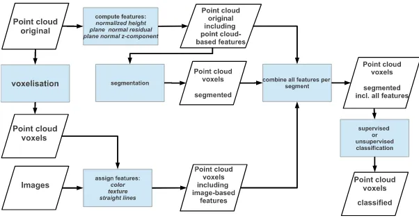
The workflow of processes within the method we propose is sket-ched in Fig. 1. The input is given by the point cloud data as de-rived from image matching, its voxel representation and the origi-nal images. Features are computed from the point cloud and from the images and assigned to each voxel. Ultimately we are aim-ing at classifyaim-ing segments which are defined by geometric fea-tures. To this end we first perform a region growing algorithm, introduced by Vosselman et al. (2004), yielding a segmentation according to planarity of segments. All voxels not assigned to a planar segment are clustered through a connected components analysis and each cluster is treated as independent segment in the following. The segmentation information is then assigned to the voxels and feature values are computed per segment. We use two different independent classification schemes: a supervised approach, based on Random Trees (RTree, (Breiman, 2001)), and an unsupervised, rule-based approach which applies a graph cut-based optimization scheme.
3.1 3D geometry- and image-based features
Points from image matching explicitly represent the geometry of objects. Man-made objects are mainly composed out of planar faces, as opposed to natural surfaces like trees and shrub. In ad-dition the height above the ground surface helps to distinguish building roofs and trees from ground. So, beside the normal-ized height, computed in the pre-processing step, we estimate per point the normal of a face, composed out of the 10 closests points. In particular we use the residual of the normal, which helps to distinguish smooth from rough surfaces. The residual of the normal corresponds to the smallest eigenvalue of the co-variance matrix associated with the centre of gravity, computed from all points under consideration; the normal vector is the cor-responding eigenvector. The Z-component of the normal is used as well in order to distinguish horizontal from vertical and other planes.
Concerning image-based features we compute color values (Hue, Saturation, in this case), texture in the form of a standard devia-tion in a 9x9 matrix around each image pixel, and straight lines. The latter one is computed using the line growing algorithm by Burns et al. (1986). For each image pixel which is part of a
tures are assigned to the correct voxel when we back project the voxel to image space. Since we have overlapping images, values for a certain feature will be observed in multiple images. There-fore, the final feature value will be computed from the median of all input values.
3.2 Combination of features per segment
We use the segment as the main entity for classification, so we need to compute per feature a joint value representing all voxels inside this segment. To this end we compute a mean value per fea-ture, associated to each segment. Further we compute a standard deviation which is used as weight in the optimization-based clas-sification. To summarize the following features are available per segment: Thenormalized heighthelps to distinguish ground from non-ground segments, thez-component of plane normalhelps to distinguish horizontal from slanted or vertical planes (fac¸ades), theresidual of plane normalis a measure for segment roughness. In addition we use2 color features: hue, saturation, thestandard deviation in a 9x9 window, which is a texture measure and related to surface properties, and finally we usestraight line length and directionwhich provide evidence for man-made structures.
3.3 Supervised segment classification using Random Trees
One of the objective of this paper is to compare the performance of a supervised classification approach and an optimization tech-nique which does not need training information, using the same features.
Two state-of-the-art machine learning techniques which showed good results in our previous experiments (Gerke, 2011) are adap-tive boosting ”AdaBoost” (Freund and Schapire, 1996) and Ran-dom Trees (Breiman, 2001). Because of the similar results ob-tained earlier we believe that the actual selection of a supervised method is not very critical here, so we chose the RTrees approach for the processing to leave space for the actual comparison bet-ween supervised and un-supervised methods in the result section.
Figure 1: Entire workflow from point clouds and images to classification
3.4 Fully automatic classification in a MRF framework
The advantage of this scheme over other techniques is that it com-bines observations (data term) with a neighborhood smoothness constraint. Among a selection of optimization methods to mini-mize the overall energy, the graph cut (Boykov et al., 2001) ap-proach showed good performance in the past. The representa-tion is in the 3D lattice, i.e. each voxel will retrieve an individual label, and thus also an individual data term and the neighbor-hood is defined in the 3D lattice, as well. However, in order to represent the segmentation the features as computed per segment will be used for the respective voxels inside. We compute energy data terms for the classesroof, tree, fac¸ade, vegetated ground, sealed ground and roof destroyed/rubbleand also add a class background to represent ”empty” voxels. In the following the classroof destroyed/rubblewill be namedrubble.
The totalEenergy is composed out of the data term and a pair-wise interaction term:
fp.Vpqis the pairwise interaction potential, considering the
neigh-borhoodN. In particular we use the Potts interaction potential as proposed by Boykov et al. (2001) which adds a simple label smoothness term:
Features contributing to the data term are normalized to the range
[0,1]. Internally all features are stored in 8bit images, i.e. in a resolution of1/256. Especially for height values this is the reducing factor, and needs to be taken into account. The feature values contribute to factors for the total energy, depending on the actual class. Each factorSis initialised with 1 to avoid that in
case a feature does not contribute evidence for a particular class the total energy vanishes. The features and the derived factors are defined as follows:
Normalized HeightmH: the normalized height coded in
decime-terdm. In order to reflect the fact that ground objects have a low height, and – depending on the object type – roofs or trees have a significantly large height above terrain we compute some valuesmHx =|mH−x|. The fact that we can store only 256
different values means that we can represent normalized heights up to25.5m. All heights above this value are set to that maxi-mum. For our task this does not restrict the functionality since the
normalized height is basically used to differentiate ground from non-ground features only.
Note: The heigt is defined indm, hence the energy formulation for roofs is in this example best for buildings up to9m, but can easily extended for taller buildings. For rubble we cannot really use knowledge concerning its normalized height. It can be close to ground, or form a relatively tall rubble pile.
Line LengthmL−andmL+: if one or more lines are assigned to the segment where the voxel is located, we compute two different values:mL−the difference to the shortest line in the overall area andmL+: the difference to the longest line. Those two values are used in the energy computation, depending on the class assuming that longer lines can be found at man-made structures, shorter lines in natural environments or at destroyed buildings.
SL= (
mL+, iffp∈ {roof,fac¸ade}
mL−, else
Plane Normal, Z-componentmZ: to distinguish horizontal from
vertical and other planes
Note: Fortree, vegetated groundandrubblethe normal vector cannot contribute any evidence – it is arbitrary. In order to avoid that this ignorance has an influence on the total energy, the factor for those classes is the same as the minimum energy from the other classes, with an added very small constant energyC.
Texture: Standard DeviationmT: standard deviation in a sliding
9x9 window in an image. Since we assume a large value for trees we also compute the overall maximum standard deviation
mT max. For tree and rubble we expect lartemTvalues.
ST = (
|mT−mT max|, iffp∈ {tree,rubble}
∗
: For the sake of simplicity the fixed angular values are given in the original unit. In practice they are also scaled to [0,1].
-To consider the uncertainty inherent in the feature values result-ing from the mergresult-ing of values from different views we add a to each factora penalizing energy which is proportional to the stan-dard deviation computed during the merge of feature values per segment.
In conclusion each feature contributes to a final factorS′
=
S+Spenper object class, which is defined in [0,1]. The energy computed from all features voting for a certain labelpis
Dp(fp) = S
In the practical implementation of graph cut we need to con-vert the energies into integer values. Some internal experiments showed that an actual ranking of the energy per entity gives the best result. That is, we assign an energy defined in[0, N−1]– whereN is the number of classes – toDp(fp), according to the
sequence in the originalDp(fp)computation.
4 RESULTS
4.1 Haiti test area
In our experiments we concentrated on the same test area as de-scribed in (Gerke and Kerle, 2011; Gerke, 2011). Pictometry1
images were acquired over Port-au-Prince, Haiti, in January 2010 a few days after the earthquake. The ground sampling distance (GSD) varies from10cmto16cm(fore- to background). Due to varying image overlap configuration the number of images which observe a particular part of the scene varies from 4 to 8. In this experiment only oblique images were used since the nadir ima-ges are shipped only after ortho rectification, and without further specification of the ortho image production process. See Fig. 2 for some example images and results. Opposed to the experi-ments conducted earlier we are now using more images (11 in-stead of only 3). Earlier we only used three images to directly compare per-image to object space classification. Here we con-centrate only on the object space and thus exploit all the informa-tion we have.
4.1.1 RTrees result The confusion table showing the RTrees classification per-segment result using the validation subset of the reference data is given in Table 1. Percentages refer to the total number of reference entities, i.e. rows sum up to 100% (±because of round-off errors). The overall classification accuracy – com-puted as the normalized trace of the confusion matrix – is 73.1%.
1http://www.pictometry.com
Tree 0.049 0.049 0.024 0.024 0.854
Table 1: Confusion matrix RTrees Haiti, overall accuracy 73.1%
Compared to the result published earlier we obtain similar results for all classes except fortree, which has a correctness here of 85% while it was much worse earlier (around 25% only). Two reasons might explain this. First, in the earlier work we did not use the normalized height explicitly, and second, the use of mul-tiple images renders more trees visible as before.
4.2 Unsupervised result
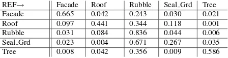
The per-voxel result from the unsupervised, MRF-based method for the Haiti testdata is shown in the confusion matrix in Table 2. Here the problem of the unclear object class definition forrubble becomes even more obvious than in the supervised result. Each object class got labeled asrubbleby at least 24% (building), and up to 67% (sealed ground). Another reason for classification er-rors is relating to the height normalization, and in particular the ground filtering. Especially in destroyed areas, for instance at rubble piles, there is a kind of smooth transition between ground and non-ground features, and the latter ones might then get la-beled as ground. This is observable in the results as well: actually 12% of all roof voxels got labeled assealed grnd. The major dif-ferentiation in the energy function for those two classes is made from the normalized height. In the result from the supervised me-thod that problem does not become this obvious since the height uncertainty gets implicitly modeled during RTrees training.
REF→ Facade Roof Rubble Seal Grd Tree
Facade 0.665 0.042 0.243 0.030 0.021
Roof 0.097 0.441 0.344 0.118 0.001
Rubble 0.031 0.084 0.836 0.044 0.006
Seal Grd 0.023 0.004 0.671 0.267 0.035
Tree 0.008 0.042 0.356 0.009 0.586
Table 2: Confusion matrix unsupervised through MRF/graph cut Haiti, overall accuracy 58.9%
4.3 Enschede test area
To use the Haiti data for the experiments has the drawback that object classes in the scene after a major seismic event are not as clearly definable as in an intact region. For this reason we will also demonstrate the new method in a dataset showing a typical European sub-urban scene. The images over Enschede were ac-quired by Slagboom en Peeters2 in May 2011. This company
mounted five Canon EOS 5D Mark II cameras in one head, using the sameMaltese Crossconfiguration as Pictometry: one camera pointing into nadir direction and the remaining ones into the four cardinal directions under a tilt angle of45◦
. Due to the low flight altitude of 500mabove ground the GSD varies from 5 to 8cm, and the image overlap is at least 60% in all directions, i.e. making
Figure 2: Example oblique images from Port-au-Prince and derived information. Upper row: oblique images facing North, East, West direction. Lower row: colored point cloud computed with PMVS2 (Furukawa and Ponce, 2010), the same with grey values representing height, zoom in to an example area, result from supervised classification, result from MRF-based classification. Images: ©Pictometry, Inc.
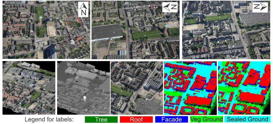
Figure 3: Example oblique images and derived information for Enschede. Upper row: oblique images facing North, East, West direction. Lower row: colored point cloud computed with PMVS2, the same with grey values representing height, zoom in to an example area, result from supervised classification, result from MRF-based classification. Images: ©Slagboom en Peeters B.V.
stereo overlap available from all perspectives. Residuals at check points are quite large, they are in the range of more than 2 pixels (RMSE up to 20cm), which also has an effect on the point cloud computation; the standard deviation computed from plane fitting residuals partly goes up to50cm, see (Xiao, 2013) for a more detailed evaluation. In Fig. 3 some example images showing the area are displayed in the upper row. The scene shows some quite large industrial halls, but also a typical settlement area with in-dividual free standing houses of different construction type. The bottom row shows the colored point cloud of the entire test area, first real colors, then a gray coded height visualisation. The centre image shows a zoom-in to a region of interest and the two right hand images give again the classification result (RTrees next to the middle image, MRF-based right hand).
4.3.1 RTrees result The confusion matrix in Table 3 shows better overall accuracy compared to the Haiti dataset; it is almost 85%. Remarkable is again the confusion of roofs and fac¸ades: 12% of fac¸ades got labeled as roof which is mainly due to small structures at facades like extensions with a flat roof structure,
which arefac¸adein the reference, but got classified asroof. More-over segments in the upper part of fac¸ades are often classified as roof due to the height. Another main confusion concerns trees and ground vegetation: more than 14% of tree-segments got la-beledveg grnd. In this case the quite fuzzy definition of those classes causes most of the confusion: close-to-ground vegetation like bushes is labeled by the operator as ground vegetation, how-ever, due to their elevation the classifier might confuse it with trees. Since we do not have access to infrared channels in this case the classifier cannot make use of spectral information to fur-ther separate those classes. This is also the reason for a certain interclass-confusion between sealed and vegetated ground seg-ments.
4.4 Unsupervised result
ten-tures to support the discrimination between sealed and vegetated ground.
REF→ Facade Roof Seal Grd Veg Grd Tree
Facade 0.628 0.231 0.073 0.051 0.018
Roof 0.066 0.838 0.071 0.006 0.020
Seal Grd 0.002 0.001 0.800 0.196 0.000
Veg Grd 0.000 0.000 0.029 0.968 0.003
Tree 0.012 0.045 0.037 0.303 0.602
Table 4: Confusion matrix unsupervised through MRF/graph cut Enschede, overall accuracy 78.3%
5 DISCUSSION AND CONCLUSIONS
We have developed and tested two different 3D scene classifica-tion methods; one was a supervised scheme, based on the Ran-dom Trees machine learning technique. The second one was for-mulated in a MRF framework, where the graph cut approach was used for energy minimization. All in all most of the results can be considered satisfactory, however, there are some specific prob-lems. If object classes are not clearly defined, that is they sig-nificantly share properties with other classes, like rubble in our example, the MRF-based method basically fails. The relatively good result for the same method, but in a better structured envi-ronment shows that such unsupervised optimization method are applicable in real-world scenarios. In fact, in that case the overall accuracy is only worse by 6% compared to the supervised me-thod. We assume that the quite noisy point cloud from the image matching has also an impact on the classification quality, at least for the unsupervised method. Thus in further work we need to have a closer look into that. A problem inherent in the approach is its overall dependency on the 3D point cloud accuracy and com-pleteness: if parts of the scene are not represnted in the point-cloud, e.g. because of poor texture, the respective area does not get considered at all. This is a drawback and would need some attention in the future.
Apart from that the whole classification will potentially become more accurate in the future. Upcoming multiple camera heads like Hexagon/Leica RCD30 Oblique or Microsoft Osprey will have NIR channels available which will make the vegetation clas-sification much simpler as in our case where only RGB was avai-lable. In addition the mid-frame cameras used in those systems are supposed to have a more stable camera geometry and better lenses compared to the DSLR cameras employed here.
ACKNOWLEDGEMENTS
Pictometry Inc. provided the dataset over Haiti. Slagboom en Peeters B.V. provided the Enschede data. We made use of the implementation of graph cut optimization by Boykov and Kol-mogorov (2004). We thank the anonymous reviewers for their valuable comments.
Breiman, L., 2001. Random forests. Machine Learning 45(1), pp. 5–32.
Burns, J., Hanson, A. and Riseman, E., 1986. Extracting straight lines. IEEE Transactions on Pattern Analysis and Machine In-telligence 8(4), pp. 425–455.
Freund, Y. and Schapire, R. E., 1996. Experiments with a new boosting algorithm. In: Machine Learning: Proceedings of the Thirteenth International Conference, Morgan Kauman, p. 148156.
Furukawa, Y. and Ponce, J., 2010. Accurate, dense, and robust multi-view stereopsis. IEEE Transactions on Pattern Analysis and Machine Intelligence 32(8), pp. 1362–1376.
Gerke, M., 2011. Supervised classification of multiple view ima-ges in object space for seismic damage assessment. In: Lecture Notes in Computer Science: Photogrammetric Image Analysis Conference 2011, Vol. 6952, Springer, Heidelberg, pp. 221– 232.
Gerke, M. and Kerle, N., 2011. Automatic structural seis-mic damage assessment with airborne oblique pictometry ima-gery. Photogrammetric Engineering and Remote Sensing 77(9), pp. 885–898.
Haene, C., Zach, C., Cohen, A., Angst, R. and Pollefeys, M., 2013. Joint 3d scene reconstruction and class segmentation. In: IEEE Conference on Computer Vision and Pattern Recognition (CVPR).
Ladick´y, L., Sturgess, P., Russell, C., Sengupta, S., Bastanlar, Y., Clocksin, W. and Torr, P., 2012. Joint optimization for object class segmentation and dense stereo reconstruction. Interna-tional Journal of Computer Vision 100(2), pp. 122–133.
Lafarge, F. and Mallet, C., 2012. Creating large-scale city mo-dels from 3d-point clouds: A robust approach with hybrid re-presentation. International Journal of Computer Vision 99(1), pp. 69–85.
Nyaruhuma, A. P., Gerke, M., Vosselman, G. and Mtalo, E. G., 2012. Verification of 2D building outlines using oblique air-borne images. ISPRS Journal of Photogrammetry and Remote Sensing 71, pp. 62–75.
Rapidlasso, 2013. Homepage lastools. http://lastools.org.
Vosselman, G., Gorte, B., Sithole, G. and Rabani, T., 2004. Recognising structure in laser scanner point clouds. In: In-ternational Archives of Photogrammetry, Remote Sensing and Spatial Information Sciences, Vol. 36number 8/W2, pp. 33–38.