THE APPLICATION OF A CAR CONFIDENCE FEATURE FOR THE CLASSIFICATION
OF CROSS-ROADS USING CONDITIONAL RANDOM FIELDS
S. G. Kosova
, F. Rottensteinera∗, C. Heipkea
, J. Leitloffb
, and S. Hinzb
a
Institute of Photogrammetry and GeoInformation, Leibniz Universit¨at Hannover, Germany {kosov, rottensteiner, heipke}@ipi.uni-hannover.de
b
Institute of Photogrammetry and Remote Sensing, Karlsruhe University of Technology, Germany {Jens.Leitloff,[email protected]}@kit.edu
Commission III WG III/4
KEY WORDS:Conditional Random Fields, Contextual, Classification, Crossroads
ABSTRACT:
The precise classification and reconstruction of crossroads from multiple aerial images is a challenging problem in remote sensing. We apply the Conditional Random Fields (CRF) approach to this problem, a probabilistic model that can be used to consider context in classification. A simple appearance-based model is combined with a probabilistic model of the co-occurrence of class label at neighbouring image sites to distinguish classes that are relevant for scenes containing crossroads. The parameters of these models are learnt from training data. We use multiple overlap aerial images to derive a digital surface model (DSM) and a true orthophoto without moving cars. From the DSM and the orthophoto we derive feature vectors that are used in the classification. Within our framework we make use of a car detector based on support vector machines (SVM), which delivers car probability values. These values are used as additional feature to support the classification when the road surface is occluded by static cars. Our approach is evaluated on a dataset of airborne photos of an urban area by a comparison of the results to reference data. The evaluation is performed for images of different resolution. The method is shown to produce promising results when using the car probability values and higher image resolution.
1 INTRODUCTION
The automatic detection and reconstruction of roads has been an important topic of research in Photogrammetry and Remote Sens-ing for several decades. Considerable progress has been made, but the problem has not been finally solved. The EuroSDR test on road extraction has shown that road extraction methods are ma-ture and reliable under favourable conditions, in particular in ru-ral areas, but they are far from being practically relevant in more challenging environments as they exist in urban or suburban ar-eas (Mayer et al., 2006). One of the main rar-easons for failure of road extraction algorithms in that test was the existence of cross-roads, due to the fact that model assumptions about roads (e.g., the existence of parallel edges delineating a road) are hurt there. For this reason, specific models for the extraction of crossroads from images have been developed. (Barsi and Heipke, 2003) used neuronal networks for a supervised per-pixel classification of greyscale orthophotos in order to detect areas corresponding to crossroads, combining radiometric and geometric features. How-ever, only examples for rural areas were shown. (Ravanbakhsh et al., 2008b, Ravanbakhsh et al., 2008a) used a model based on snakes to delineate outlines of road surfaces at crossroads, includ-ing the delineation of traffic islands. The main reasons for failure of that method were occlusion of the road surface by cars and a complex 3D geometry, e.g. at motorway interchanges. Occlu-sions were also a major problem in (Grote et al., 2012), which also gives an overview over other current road detection tech-niques. The problem of occlusion by cars could be overcome if the position of cars were known in the images.
Conditional Random Fields (CRF) can be used for a raster-based classification of images (Kumar and Hebert, 2006). CRF offer probabilistic models for including context in the classification process by considering the statistical dependencies between the class labels at neighbouring image sites. Nevertheless, their
ap-∗Corresponding author
i.e. each object on higher level interacts with its smaller parts on lower level. In (Winn and Shotton, 2006), the part-based model is motivated by the methods potential to incorporate information about the relative alignment of object parts and to model longe-range interactions. However, occluded objects are not explicitly reconstructed. The spatial structure of such part-based models is not rotation-invariant and, thus, requires the availability of a ref-erence direction (the vertical in images with a horizontal viewing direction), not available in aerial imagery. In (Wojek and Schiele, 2008), a CRF having several layers is used, but the additional layer is related to a label for object identity, used to track an ob-ject detected by a specific obob-ject detector over several images.
In (Kosov et al., 2013) we did already propose a two-layer CRF to deal with occlusions, but the classifier used for the associa-tion potentials was based Gaussian mixture models and no car confidence feature was applied. The method presented in this pa-per applies a better base classifier for the association potentials, namely Random Forests (RF), and again includes the car confi-dence features. The main advantage of separating two class labels is a better potential for correctly classifying partly occluded areas while maintaining the occluding objects such as cars or trees. Our method is evaluated using 90 crossroads of the Vaihingen data set of the German Society of Photogrammetry, Remote Sensing and Geoinformation (DGPF). We use image and DSM data having a ground sampling distance (GSD) of 8 cm. The focus of the eval-uation is on the impact of the car confidence feature, the context model, and the image resolution on the results.
2 CONDITIONAL RANDOM FIELDS (CRF)
We assume an imageyto consist ofMimage sites (pixels or seg-ments)i∈Swith observed datayi, i.e.,y= (y1,y2, . . . ,yM)
T
, whereSis the set of all sites. With each siteiwe associate a class labelxifrom a given set of classesC. Collecting the
la-belsxiin a vectorx = (x1, x2, . . . , xM)T, we can formulate
the classification problem as finding the label configurationˆxthat maximises the posterior probability of the labels given the obser-vations,p(x|y). A CRF is a model ofp(x|y)with an associated graph whose nodes are linked to the image sites and whose edges model interactions between neighbouring sites. Restricting our-selves to a pairwise interactions,p(x|y)can be modelled by (Ku-mar and Hebert, 2006): action potentialsmodelling the dependencies between the class labels at two neighbouring sitesiandjand the datay,Niis the
set of neighbours of sitei(thus,jis a neighbour ofi), andZis a normalizing constant. Applications of the CRF model differ in the way they define the graph structure, in the observed features, and in the models used for the potentials. Our adaptations of the framework will be explained in Section 3.
3 METHOD
The goal of our method is the pixel-based classification of ur-ban scenes containing crossroads. The primary input consists of multiple aerial images and their orientation data. We require at least fourfold overlap of each crossroads from two different im-age strips in order to avoid occlusions as far as possible. In a preprocessing stage, these multiple images are used to derive a
DSM by dense matching. The DSM is used to generate a true or-thophoto from all input images, taking advantage of the multiple views to eliminate moving cars. More details about the prepro-cessing stage can be found in (Kosov et al., 2012). The DSM and the combined orthophoto are the input for extracting the features, which provide the input to the CRF-based classifier.
3.1 Twin CRF
In this paper we split objects corresponding to thebase level, i.e. the most distant objects that cannot occlude other objects but could be occluded, and objects corresponding to theocclusion level, i.e. all other objects. This implies that, two class labels xb
i ∈Cbandxoi ∈Coare determined for each image sitei. They
correspond to the base and occlusion levels, respectively;Cband
Co
are the corresponding sets of class labels withCbTCo =∅
. In our application,Cbconsists of classes such asroadorbuilding, whereasCoincludes classes such ascarandtree. Coincludes a special classvoid∈Co
to model situations where the base level is not occluded. We model the posterior probabilitiesp(xb|y), p(xo
|y)directly, expanding the model in Eq. 1:
p(xb,xo|y) = 1 In Eq. 2, the association potentialsϕl
i, l ∈ {o, b}link the data
ywith the class labelsxliof image site iat levell. The
inter-action potentials ψl
ij, l ∈ {o, b}, model the dependencies
be-tween the datayand the labels at two neighbouring sitesiandj at each level. This model implies that the two levels do not in-teract. Training the parameters of the potentials in Eq. 2 requires fully labelled training images. The classification of new images is carried out by maximizing the probability in Eq. 2.
3.1.1 Association Potential: Omitting the superscript indicat-ing the level of the model, the association potentialsϕi(xi,y)are
related to the probability of a labelxitaking a valuecgiven the
data yby ϕi(xi,y) = p(xi = c|fi(y))(Kumar and Hebert,
2006), where the image data are represented by site-wise feature vectorsfi(y)that may depend on all the observationsy. Note that
the definition of these feature vectors may vary with the dataset. We use a Random Forest (RF) (Breiman, 2001) in the implemen-tation of (OpenCV, 2012) for the association potentials both of the base and for the occlusion levels, i.e.ϕb
i(xbi,y)andϕoi(xoi,y).
A RF consists ofNTdecision trees that are generated in the
train-ing phase. In the classification, each tree casts a vote for the most likely class. If the number of votes cast for a classcisNc, the
probability underlying our definition of the association potentials isp(xi=c|fi(y)) =Nc/NT.
3.1.2 Interaction Potential: This potential describes how likely a pair of neighbouring sitesiandj is to take the labels
(xi, xj) = (c, c′)given the data:ψij(xi, xj,y) =p(xi=c, xj = c′|y)(Kumar and Hebert, 2006). We generate a 2D
his-togramh′
ψ(xi, xj)of the co-occurrence of labels at neighbouring
sites from the training data;h′ψ(xi =c, xj =c′)is the number
of occurrences of the classes(c, c′)at neighbouring sitesiand j. We scale the rows ofh′
ψ(xi, xj)so that the largest value in a
In Eq. 3,λ1 andλ2 determine the relative weight of the inter-action potential compared to the association potential. As the largest entries ofhψ(xi, xj)are usually found in the diagonals,
a model without the data-dependent term in Eq. 3 would favour identical class labels at neighbouring image sites and, thus, re-sult in a smoothed label image. This will still be the case if the feature vectorsfiandfjare identical. However, large differences
between the features will reduce the impact of this smoothness as-sumption and make a class change between neighbouring image sites more likely. This model differs from the contrast-sensitive Potts model (Boykov and Jolly, 2001) by the use of the nor-malised histogramshψ(xi, xj)in Eq. 3. It is also different from
methods such as those described in (Rabinovich et al., 2007), who use the co-occurrence of objects in a scene to define aglobalprior to make the detection of small objects in a scene more likely if related larger objects are found. We use the co-occurrence of neighbouringobjects to favourlocallabel transitions that occur more frequently in the training data. Again, the training of the models for the base and the occlusion levels,ψb
ij(xbi, xbj,y)and ψo
ij(xoi, xoj,y), respectively, are carried out independently from
each other using fully labelled training data.
3.2 Car Detection
The presence of vehicles in optical images is a strong indicator for roads. Thus a seperate classifcation of cars seem to be very useful for reconstruction of crossroads. A very similar idea was already shown in (Hinz, 2004). There, hierachical wire-frame models were used for the verification of already detected roads. In general, vehicle detection is performed either using implicit or explicit models. Extensive overviews of previous work can be found in (Stilla et al., 2004) and (Hinz et al., 2006).
The directions of the roads are unknown in advance. Thus, we also use HOG features. These image features can be calculated very efficiently by integral histograms (Porikli, 2005) for the slid-ing classification windows. The window size is80×80 pix-els. We calculate histograms with 9 bins for 100 non-overlapping blocks of8 × 8pixels each. Training and classification is per-formed using nonlinear Support Vector Machines (SVM) with soft margins and radial basis functions as kernel. The kernel parameter and error weight of slack variables is determined by cross-validation on the training data. The membership of each pixelito classcargiven its feature vectoryiis calculated by
f(yi) =sign
wTϕ(yi)
(4)
wherewis the normal vector andbthe vertical distance to feature space origin of the seperating hyperplane in the tranformed fea-ture space. Transformation of feafea-ture vectors is given by the tran-formϕ(yi). This function only gives a binary decision, which is
not suitable as an input for the CRF. Thus, posteriori probabili-tiesP(xi|yi)for each pixeliare estimated. For that purpose,
the posterior is approximeted by a sigmoid function as proposed by (Platt, 2000):
P(xi=car|y)≈PA,B[f(yi)] =
1
1 + exp [A(yi) +B]
(5) The parametersAandBare estimated by the algorithm given in (Lin et al., 2007), which is more robust than the original algo-rithm of (Platt, 2000).
3.3 Definition of the Features
As stated in Section 3.1.1, we derive a feature vectorfi(y)for
each image siteithat consists of seven features derived from the
orthophoto (image features) collected in a vectorfimg, a feature
derived from the DSM (fDSM) and, optionally, the car
confi-dence feature (fcar), defined as the posterior in Eq. 5. We also
make use of multi-scale features, collected in a vectorfM S. The
site-wise feature vectors are fi(y)T = (fTimg, fDSM,fTM S) or
fi(y)T = (fTimg, fDSM,fTM S, fcar), depending on whether the
car confidence feature is used or not. For numerical reasons all features are scaled linearly into the range between0and255and then quantized by8bit.
We do not use the colour vectors of the images directly to define the site-wise image feature vectorsfimg. The first three features
are the normalized difference vegetation index (N DV I), derived from the near infrared and the red band of the CIR orthophoto, the saturation (sat) component after transforming the image to the LHS colour space, and image intensity (int), calculated as the average of the two non-infrared channels. We also make use of the variance of intensity (varint) and the variance of saturation
(varsat), determined from a local neighbourhood of each pixel
(7 ×7pixels forvarint,13 ×13pixels forvarsat). The sixth
image feature (dist) represents the relation between an image site and its nearest edge pixel; this feature should model the fact that road pixels are usually found in a certain distance either from road edges or road markings. We generate an edge image by threshold-ing the intensity gradient of the input image. Then, we determine a distance map from this edge image. The feature used in classi-fication is the distance of an image site to its nearest edge pixel, taken from the distance map. Thus, the image feature vector for each pixel isfimg= (N DV I, sat, int, varsat, varint, dist)T.
A coarse Digital Terrain Model (DT M) is generated from the DSM by applying a morphological opening filter with a struc-tural element whose size corresponds to the size of the largest off-terrain structure in the scene, followed by a median filter with the same kernel size. TheDSMfeature is the difference between theDSMand theDT M, i.e.,fDSM =DSM −DT M. This
feature describes the relative elevation of objects above ground such as buildings, trees, or bridges. The multi-scale featuresfM S
comprise theN DV I,fDSMandsatfeatures, calculated at two
coarser different scales as average values in squares of21×21
and49×49pixels, respectively.
3.4 Training and Inference
Training of a CRF is computationally intractable if to be car-ried out in a probabilistic framework (Kumar and Hebert, 2006). Thus, approximate solutions have to be used for training. In our application, we determine the parameters of the association and interaction potentials separately based on fully labelled training images. The RF classifier used in the association potentials are trained using the site-wise feature vectors of the training images. The interaction potentials are derived from scaled versions of the 2D histograms of the co-occurrence of class labels at neighbour-ing image sites in the way described in Sec. 3.1.2, takneighbour-ing into account all image sites in the training data. The parametersλ1 andλ2in the Eq. 3 are set manually to values2.0and0.01, re-spectively. Exact inference is also computationally intractable for CRFs. We use Loopy Belief Propagation (LBP), a standard tech-nique for probability propagation in graphs with cycles that has shown to give good results in the comparison reported in (Vish-wanathan et al., 2006).
4 EXPERIMENTS
4.1 Experimental Setup
(a) (b)
Figure 1: Posterior probability from SVM classification. (a) orig-inal image, (b) classification result.
(a) (b)
Figure 2: Results of blurred vehicle caused by median filtering. (a) original image, (b) classification result.
for our experiments. For each crossroads, a true orthophoto and a DSM were available, each covering an area of80 ×80m2
with a GSD of 8 cm. The DSM and the orthophoto were generated from multiple aerial CIR images in the way described in (Kosov et al., 2012). They provide the original input to our CRF-based classifier. We defined each image site to correspond to image pixels, thus in the full resolution each graphical model consisted of1000×1000nodes. The neighbourhoodNiof an image site iin Eq. 1 is chosen to consist of the direct neighbours ofiin the data grid.
We defined six classes that are characteristic for scenes contain-ing crossroads, namelyasphalt(asp.),building(bld.),tree,grass (gr.),agricultural(agr.) andcar, so thatCb={asp.,bld.,gr.,agr.} andCo ={tree,car,void}
. The two-level reference was gener-ated by manually labeling the orthophotos using these 6 classes, using assumptions about the continuity of objects such as road edges in occluded areas to define the reference of the base level.
For the evaluation we used cross validation. In each test run, 45 images were used for training, and the remaining 45 for testing. This was repeated two times so that each image was used first for training and second for testing. The results were compared with the reference; we report the completeness and the correctness of the results per class as well as the overall accuracy (Rutzinger et al., 2009).
4.2 Car Detection
Classification gives the probability for vehicles for each pixel. In case of cleary seperated cars, the approach delivers results as illustrated in Fig. 1. During image generation moving vehicles should be eliminated. Still, several ”blurred” vehicles are still visible. These vehicles also give response during classification, even so, the probabilties are smaller than 1 due to low contrast. An example is given in Fig. 2. Furthermore, objects of similar dimension recieve high probalities as it can be seen in Fig. 3.
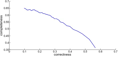
In Fig. 4 the completeness versus correctness for different thresh-olds on the estimated vehicle probalities are shown. For this eval-uation, the centre point of connected pixel having a larger value
(a) (b)
Figure 3: Results of vehicle-like image parts. (a) original image, (b) classification result.
0 0.1 0.2 0.3 0.4 0.5 0.6 0.7
0.35 0.4 0.45 0.5 0.55 0.6 0.65 0.7
correctness
completeness
Figure 4: ROC for variying thresholds of probability.
than the threshold is compared to the regions of the reference (e.g. first row of Fig. 5). Thus, connected regions which cover multiple vehicles (e.g. last row of Fig. 5) are only counted once and lead to a signifcant reduction of completeness. Therefore, the given value for completeness in Fig. 4 are quite pessimistic. Nev-ertheless, the overall correctness still needs further improvement, which could be achieved by additional features and an additional classification of the connected regions. This is planed for future work.
4.3 Results and Discussion
We carried out eight experiments. In the first four experiments (RF5
car,RF 5
,CRF5 car,CRF
5
) we used a version of the Vaihin-gen dataset with a reduced GSD of 40 cm (corresponding to 5×5 pixels of the original images), so that the CRF only consisted of 200×200 nodes. In the second set of experiments (RF1
car,RF 1
, CRF1
car,CRF 1
) we used the images at their full resolution of 8 cm. In the experimentsRF1
carandRF 5
car, we only used the
Random Forest classifier for a local classification of each node, neglecting the interaction potentials. In the experimentsCRF1
car
andCRF5
car, the twin CRF model in Eq. 2 was used, including
the interactions. The experimentsRF5 car,CRF
5 car,RF
1 car and CRF1
carwere performed using the car confidence feature, while
for the experimentsRF5 ,CRF5
,RF1
andCRF1
the car con-fidence feature was not applied. The completeness and the cor-rectness of the results achieved in these experiments are shown in Tab. 1 and 2. For the occlusion layer we also report the qual-ity (Rutzinger et al., 2009), which is a measure for the trade-off between completeness and correcntess.
asp. bld. gr. agr. OA
RF5 car
Cm. 80.1 82.6 82.7 56.3
78.5
Cr. 84.6 78.4 79.7 62.2
CRF5 car
Cm. 82.2 76.5 89.0 42.2
79.2
Cr. 83.7 87.9 75.3 78.8
RF5 Cm. 79.8 83.8 82.9 52.9
78.3
Cr. 85.5 77.8 79.0 61.1
CRF5 Cm. 81.7 77.0 88.7 41.8
79.0
Cr. 83.7 87.2 75.3 77.1
RF1 car
Cm. 79.8 83.7 82.9 54.9
78.5
Cr. 85.5 77.6 79.4 62.0
CRF1 car
Cm. 80.7 84.5 84.7 54.7
79.6
Cr. 86.4 78.9 79.6 68.8
RF1 Cm. 79.8 83.8 82.9 52.9
78.3
Cr. 85.5 77.8 79.0 61.1
CRF1 Cm. 80.8 84.6 84.9 52.5
79.5
Cr. 86.5 79.0 79.1 68.5
Table 1: Completeness (Cm.), Correctness (Cr.), overall accu-racy (OA) [%] for the base layer.
void tree car OA
RF5 car
Cm. 77.8 85.5 75.8
79.1
Cr. 95.4 56.2 10.9 Q. 75.0 51.3 10.5
CRF5 car
Cm. 94.3 50.4 9.0
84.9
Cr. 87.8 67.7 75.5 Q. 83.4 40.6 8.7
RF5
Cm. 76.5 85.5 72.7
78.2
Cr. 95.3 55.6 9.4 Q. 73.7 50.8 9.1
CRF5
Cm. 93.9 51.8 3.5
84.8
Cr. 88.0 66.7 55.9 Q. 83.2 41.2 3.4
RF1 car
Cm. 77.5 85.6 77.6
79.0
Cr. 95.5 56.3 10.8 Q. 74.8 51.4 10.5
CRF1 car
Cm. 84.0 87.2 34.2
84.1
Cr. 95.5 57.1 41.6 Q. 80.8 52.7 23.1
RF1
Cm. 76.0 86.3 75.1
77.9
Cr. 95.5 56.2 8.9 Q. 73.4 51.6 8.6
CRF1
Cm. 83.5 87.8 32.9
83.8
Cr. 95.6 56.8 31.7 Q. 80.4 52.6 19.3
Table 2: Completeness (Cm.), Correctness (Cr.), Quality (Q.), overall accuracy (OA) [%] for the occlusion layer.
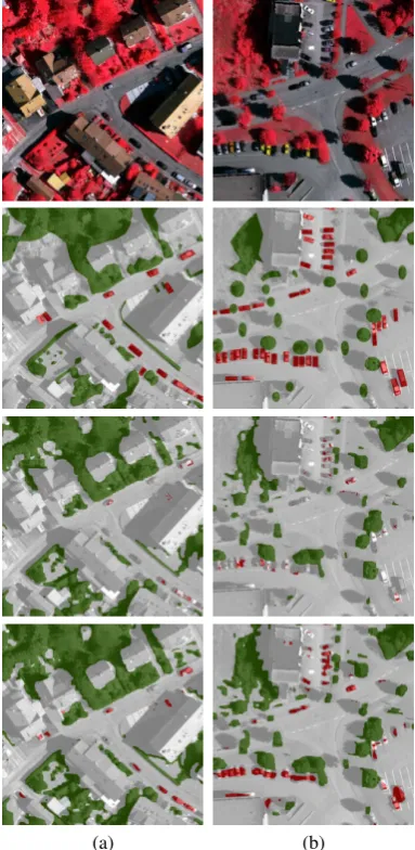
Tab. 2 shows that the occlusion layer, containing the classcar, shows a larger variation of the quality metrics between the dif-ferent experiments. The most obvious improvement is achieved by considering local context: the overall accuracy achieved in the experiments based on CRF is 5%-6% better than the one achieved in the RF experiments. This is mainly due to an improvement of the completeness of classvoid, an indicator that in the RF sce-nario there are more false positivecarand, in the lower resolu-tion,treeobjects, which is confirmed by the correctness numbers of these objects in the RF setting. Whereas the overall accuracy is similar between the experiments at full resolution and those at a reduced resolution, it becomes evident that the oversmoothing in the latter leads to a particularly poor performance for the smallest objects in our classification schemes, i.e. cars. For these objects, a classification at full resolution seems to be required.
Look-(a) (b)
Figure 5: Classification of the occlusion leyer. First row: Original images (GSD 8 cm), second row: reference, third row: CRF, fourth row:CRFcar. (a) Scene #23; (b) Scene #36. White:void;
dark green:tree; red:car.
ing at the results achieved for the images at full resolution, in the CRF setting, a better trade-off between completeness and correct-ness is achieved for the classcar, indicated by the higher quality scores (Q.in Tab. 2) compared to the RF experiments. Tab. 2 also shows that indeed the car feature helps in the classification of cars. ExperimentCRF1
car achieves the highest quality score
forcar, though there is still considerable room for improvement.
Fig. 5 illustrates two scenes with a high number of cars. Its third row presents the results ofCRF1
, while the fourth row shows results of theCRF1
carexperiment. In these scenes, using the car
confidence feature improves the classification rate for cars con-siderably. In comparison to the reference (second row of Fig. 5), cars are oversmoothed and hardly recognizable in the results of CRF1
. CRF1
cardelivers the results with the car regions in the
correct positions and nearly without false positives.
5 CONCLUSION
Distinguishing 7 classes relevant in the context of crossroads, an overall accuracy of about79-85% could be achieved. The car confidence feature, which is based on the output of our car detec-tor, is shown to increase the accuracy of classification especially for the classcar. In the future we want to improve our method by integrating more expressive features, e.g. features related to car trajectories. Furthermore, the interactions between the two levels need to be modelled in a way similar to (Kosov et al., 2013).
ACKNOWLEDGEMENTS
This research was funded by the German Science Foundation (DFG) under grants HE 1822/25-1 and HI 1289/1-1. The Vaihin-gen data set was provided by the German Society for Photogram-metry, Remote Sensing and Geoinformation (DGPF) (Cramer, 2010): http://www.ifp.uni-stuttgart.de/dgpf/DKEP-Allg.html.
REFERENCES
Barsi, A. and Heipke, C., 2003. Artificial neural networks for the detection of road junctions in aerial images. In: International Archives of the Photogrammetry, Remote Sensing and Spatial In-formation Sciences, Vol. XXXIV-3/W8, pp. 18–21.
Boykov, Y. and Jolly, M., 2001. Interactive graph cuts for opti-mal boundary and region segmentation of objects in n-d images. In: Proc. International Conference on Computer Vision (ICCV), Vol. I, pp. 105–112.
Breiman, L., 2001. Random forests. Machine Learning 45, pp. 5– 32.
Cramer, M., 2010. The DGPF test on digital aerial camera evalua-tion - overview and test design. Photogrammetrie Fernerkundung Geoinformation 2(2010), pp. 73–82.
Grabner, H., Nguyen, T., Gruber, B. and Bischof, H., 2008. On-line boosting-based car detection from aerial images. ISPRS Journal of Photogrammetry and Remote Sensing 63(3), pp. 382– 396.
Grote, A., Heipke, C. and Rottensteiner, F., 2012. Road network extraction in suburban areas. Photogrammetric Record 27, pp. 8– 28.
Hinz, S., 2004. Detection of vehicles and vehicle queues in high resolution aerial images. Photogrammetrie Fernerkundung -Geoinformation 3, pp. 201–213.
Hinz, S., Bamler, R. and Stilla, U., 2006. Theme issue: Airborne and spaceborne trafc monitoring. ISPRS J. Photogramm. & Rem. Sens. 61(3/4).
Kembhavi, A., Harwood, D. and Davis, L. S., 2011. Vehicle de-tection using partial least squares. IEEE Transactions on Pattern Analysis and Machine Intelligence 33(6), pp. 1250–1265.
Kosov, S., Rottensteiner, F. and Heipke, C., 2013. Sequen-tial gaussian mixture models for two-level conditional random fields. In: Proceedings of the 35th German Conference on Pat-tern Recognition (GCPR), LNCS, Vol. 8142, Springer, Heidel-berg, pp. 153–163.
Kosov, S., Rottensteiner, F., Heipke, C., Leitloff, J. and Hinz, S., 2012. 3d classification of crossroads from multiple aerial images using markov random fields. In: International Archives of the Photogrammetry, Remote Sensing and Spatial Information Sci-ences, Vol. XXXIX-B3, pp. 479–484.
Kumar, S. and Hebert, M., 2005. A hierarchical field framework for unified context-based classification. In: Proc. International Conference on Computer Vision (ICCV), pp. 1284–1291.
Kumar, S. and Hebert, M., 2006. Discriminative Random Fields. International Journal of Computer Vision 68(2), pp. 179–201.
Leibe, B., Leonardis, A. and Schiele, B., 2008. Robust object detection with interleaved categorization and segmentation. In-ternational Journal of Computer Vision 77, pp. 259–289.
Lin, H.-T., Lin, C.-J. and Weng, R. C., 2007. A note on platts probabilistic outputs for support vector machines. Machine learn-ing 68(3), pp. 267–276.
Mayer, H., Hinz, S., Bacher, U. and Baltsavias, E., 2006. A test of automatic road extraction approaches. In: International Archives of the Photogrammetry, Remote Sensing and Spatial Information Sciences, Vol. XXXVI-3, pp. 209–214.
OpenCV, 2012. Machine Learning.
http://docs.opencv.org/modules/ml/doc/ml.html.
Platt, J. C., 2000. Probabilistic outputs for support vector ma-chines and comparisons to regularized likelihood methods. In: A. Smola, P. Bartlett, B. Schlkopf and D. Schuurmans (eds), Ad-vances in Large Margin Classiers, MIT Press.
Porikli, F., 2005. Integral histogram: A fast way to extract his-tograms in cartesian spaces. In: Proc. Conf. Computer Vision and Pattern Recognition (CVPR), Vol. 1, IEEE, pp. 829–836.
Rabinovich, A., Vedaldi, A., Galleguillos, C., Wiewiora, E. and Belongie, S., 2007. Objects in context. In: Proceedings of the International Conference on Computer Vision (ICCV).
Ravanbakhsh, M., Heipke, C. and Pakzad, K., 2008a. Automatic extraction of traffic islands from aerial images. Photogrammetrie Fernerkundung Geoinformation 5(2008), pp. 375–384.
Ravanbakhsh, M., Heipke, C. and Pakzad, K., 2008b. Road junc-tion extracjunc-tion from high resolujunc-tion aerial imagery. Photogram-metric Record 23, pp. 405–423.
Rutzinger, M., Rottensteiner, F. and Pfeifer, N., 2009. A compari-son of evaluation techniques for building extraction from airborne laser scanning. IEEE-JSTARS 2(1), pp. 11–20.
Schindler, K., 2012. An overview and comparison of smooth labeling methods for land-cover classification. IEEE-TGARS 50, pp. 4534–4545.
Schnitzspan, P., Fritz, M., Roth, S. and Schiele, B., 2009. Dis-criminative structure learning of hierarchical representations for object detection. In: Proc. Conf. Computer Vision and Pattern Recognition (CVPR), pp. 2238–2245.
Stilla, U., Michaelsen, E., S¨orgel, U., Hinz, S. and Ender, J., 2004. Airborne monitoring of vehicle activity in urban areas. In: International Archives of the Photogrammetry, Remote Sensing and Spatial Information Sciences, Vol. XXXV- B3, pp. 973–979.
Vishwanathan, S. V. N., Schraudolph, N. N., Schmidt, M. W. and Murphy, K. P., 2006. Accelerated training of conditional random fields with stochastic gradient methods. In: Proc. 23rd ICML, pp. 969–976.
Winn, J. and Shotton, J., 2006. The layout consistent random field for recognizing and segmenting partially occluded objects. In: Proc. Conf. Computer Vision and Pattern Recognition (CVPR).