MATCHING PERSISTENT SCATTERERS TO BUILDINGS
A. Schunert*, L. Schack, U. Soergel
a Leibniz Universität Hannover, Institute of Photogrammetry and GeoInformation, Nienburger Strasse 1, 30167 Hannover, Germany - (schunert, schack, soergel)@ipi.uni-hannover.de
Commission VII, WG 2
KEY WORDS: SAR, Interferometer, Monitoring, Matching, Urban
ABSTRACT:
Persistent Scatterer Interferometry (PSI) is by now a mature technique for the estimation of surface deformation in urban areas. In contrast to the classical interferometry a stack of interferograms is used to minimize the influence of atmospheric disturbances and to select a set of temporarily stable radar targets, the so called Persistent Scatterers (PS). As a result the deformation time series and the height for all identified PS are obtained with high accuracy. The achievable PS density depends thereby on the characteristics of the scene at hand and on the spatial resolution of the used SAR data. This means especially that the location of PS cannot be chosen by the operator and consequently deformation processes of interest may be spatially undersampled and not retrievable from the data. In case of the newly available high resolution SAR data, offering a ground resolution around one metre, the sampling is potentially dense enough to enable a monitoring of single buildings. However, the number of PS to be found on a single building highly depends on its orientation to the viewing direction of the sensor, its facade and roof structure, and also the surrounding buildings. It is thus of major importance to assess the PS density for the buildings in a scene for real world monitoring scenarios. Besides that it is interesting from a scientific point of view to investigate the factors influencing the PS density. In this work, we fuse building outlines (i.e. 2D GIS data) with a geocoded PS point cloud, which consists mainly in estimating and removing a shift between both datasets. After alignment of both datasets, the PS are assigned to buildings, which is in turn used to determine the PS density per building. The resulting map is a helpful tool to investigate the factors influencing PS density at buildings.
* Corresponding author.
1. INTRODUCTION
In the last years Persistent Scatterer Interferometry (PSI) attracted a lot of attention as a tool for accurately mapping deformation on a sparse grid of temporally stable radar targets (Ferretti et al, 2000), (Hooper, 2006). Especially the possibility to completely or partially replace expensive and time consuming measurement campaigns like levelling is very appealing. In general the PS density is very high in urban areas, which is especially true if high resolution data featuring a ground resolution around one meter (for instance acquired by the TerraSAR-X satellite in High Resolution Spotlight mode) is used. According to (Gernhardt et al, 2010) densities of up to 100,000 PS per square kilometre can be achieved, which makes even the monitoring of single buildings conceivable. However, a sufficient sampling for all buildings is by no means guaranteed. While some buildings accommodate a plethora of PS, others host just few or even no points. In order to apply PSI operationally for the surveillance of urban infrastructure, it is important to determine how good a structure under investigation can be monitored with the available data. From a scientific point of view it is very interesting to investigate the circumstances leading to PS. For that purpose a map indicating the PS density per building is very helpful to identify conspicuous cases like buildings hosting unexpectedly many or few PS. A quite simple but still expressive measure is the number of PS per volume. In this work we aim to map this quantity for a test site located in the inner city area of Berlin
(Germany). The main prerequisite is an assignment of PS to buildings. For that the buildings are represented by their outlines and matched to the PS set (i.e. a residual shift between building outlines and the PS set is removed). The PS are then attributed to the closest building if their individual distance is below a threshold. Since no polyhedral 3D city model of the test site is available, the volume of every building is calculated based on a prismatic model. That is, the outline is extruded to the mean height of the building. The resulting map is finally used to select three interesting sites showing some factors, which have a strong influence on the PS density.
2. DATA
In order to determine the PS density per building, the PS point cloud is fused with map data constituting the building outlines. In the following both datasets are briefly introduced.
2.1 Persistent Scatterer
The PS results are based on processing of a stack of 20 TerraSAR-X High Resolution Spotlight images. The applied method follows the ideas presented in (Ferretti et al. 2000) and (Liu et al., 2009). A pixel of the SAR image is chosen as a PS if its phase is temporally coherent and if its amplitude is a local maximum. The former is a quite common criterion to enforce temporal stability, while the latter prevents the selection of several pixels per PS. As a result a set of temporally stable radar
targets with its 3D position and its deformation time series is obtained. In Figure 1 a 3D view of the geocoded point cloud is shown. It is quite easy to recognise the major urban structures in this point cloud. An automatic reconstruction of buildings as done with airborne laserscanning data is however quite difficult due to the irregular point distribution and the limited positioning accuracy. For that reason additional map data is used, which makes an assignment of PS to buildings possible.
2.2 Building Outlines
The GIS data used throughout this research has been digitised manually using Google EarthTM. Due to that its level of detail and accuracy is limited. However, we believe it to be sufficient for the purpose of determining the affiliation of PS to buildings. The GIS data is shown in Figure 2 overlaid to a Google EarthTM view of the scene. Internally the map data is represented as a set of polygons.
Since the data has been digitised piecewise, its level of detail as well as its accuracy are not homogeneous. In general, interior complicated buildings. The prismatic building models can be
seen in Figure 6.
3. METHODOLOGY
The compilation of a PS density map over buildings requires essentially two processing steps. First the PS point cloud and the GIS data have to be geometrically aligned. Secondly, the PS have to be assigned to the buildings. Both steps are conducted using the planimetric positions of the PS only, since no 3D GIS data like a 3D city model are available.
3.1 Geometrical alignment
The alignment of the datasets with respect to each other is necessary since both may be systematically displaced from their true position. This is especially the case for the PS point cloud due to the necessity to choose a reference PS at zero elevation. An inappropriate choice will results in a point cloud displaced in the sensors viewing direction (Gernhardt et al, 2011). Since the GIS data have been digitised using Google EarthTM, it cannot be considered accurate. However, we are just interested in a relative alignment of both datasets. Thus, the PS point cloud is shifted in order to match the map data, which is advantageous since all results are referenced to Google EarthTM by doing so. The methodology employed to estimate the misalignment between both datasets is a simplified version of the popular Iterative Closest Point algorithm (ICP) (Besl, 1992). The coordinate transformation is assumed to be a two-dimensional shift, which simplifies the ICP procedure considerably.
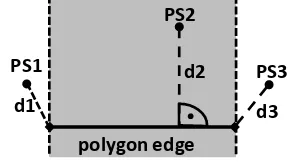
Initially PS located on building roofs and other structures within the building outlines have to be filtered out as they cannot have corresponding points in the GIS data. This is done with a filter similar to the one used in (Gernhardt et al, 2011) to remove PS located at facades. It essentially checks the height variance of all PS in a local neighbourhood around the point under investigation. If the variance exceeds a threshold, the PS is tagged as a facade PS and kept for the ICP procedure. While this is quite effective to filter out PS on building roofs and on the ground, it certainly does not remove PS at vertical structures inside the outline of the building like facades bounding interior courtyards. Those structures are in general not included in the used GIS data, which may be problematic in some cases. After filtering the ICP procedure is performed. For every point of the PS set a shift vector to the closest point in the map data is determined. The distance between a point and a polygon edge (i.e. a line segment) is defined following (Besl, 1992) and sketched in Figure 3. If the PS is located in the area shaded in grey, the distance is measured along the plumb line (PS2 with distance d2). Otherwise the distance is measured to one of the polygon points (PS1 and PS3). For every PS all edges in a certain neighbourhood are checked. Given the point correspondences a shift can be estimated which minimises the sum of the squared distances between both datasets.
Let (xi,yi) denote the coordinates of the PS set and (Xi,Yi) denote the coordinates of the set of corresponding points in the map data.
Figure 1. Geocoded PS set in 3D coordinate system. The colour codes the height
Figure 2. The used building outlines overlaid to a Google EarthTM map.
Figure 3. Definition of the distance between polygon edges and PS.
The objective function can be stated as
where Δx and Δy are the unknown shift parameters and N is the cardinality of the set of point correspondences. A local minimum of this function can be easily obtained by setting:
simply averaging the coordinate differences of all point correspondences. Finally the shift has to be applied to one of the point sets. Throughout this work the PS set is shifted, which is quite convenient for the depiction of the results in Google EarthTM.
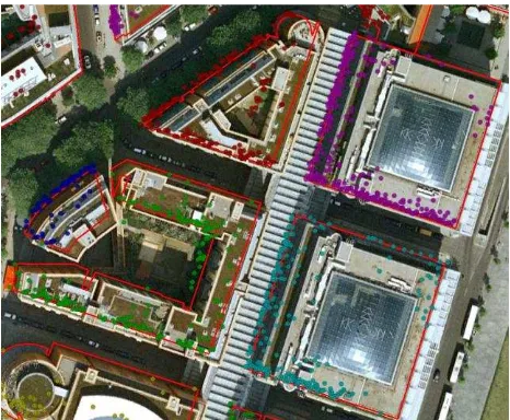
The procedure of finding the nearest neighbours, estimation, and application of the shift has to be done iteratively since the point correspondences are usually not correct in the first place. The cumulative shift (i.e. the sum of the shifts of all iterations) is finally applied to the complete PS. A subset of the PS before the application of the shift together with some building outlines overlaid to Google EarthTM is displayed in Figure 4. The same situation is shown in Figure 5 after the application of the shift. The alignment is clearly visible. The shift direction corresponds roughly with the looking direction of the SAR sensor, confirming the aforementioned assumption that the misalignment is mainly caused by an inappropriate choice of the reference PS.
3.2 Assignment of PS to buildings
After alignment of PS point cloud and GIS data, the PS can be assigned to buildings. For that a simple nearest neighbour criterion is used. For every PS the distance to polygon edges in a local neighbourhood is determined. The PS is assigned to the polygon containing the closest edge. A result of the assignment
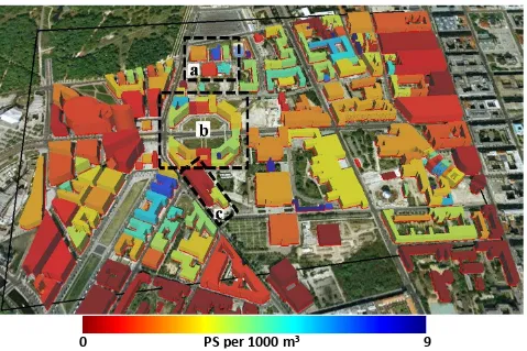
for a subset of the scene is indicated by the colours of the points in Figure 5. In the case at hand the purely geometric assignment works well, because the buildings are far enough apart. In other cases, where buildings are very close to each other, wrong assignments will emerge. However, for the sake of counting PS we assume those wrong assignments to be negligible for calculation of the volume coloured according to their PS density overlaid to Google EarthTM. The black polygon marks the area where both PS and GIS data are available. At first glance the density appears to be quite heterogeneous. While most of the buildings host not more than five PS per 1000m3 (the mean value is around three PS per 1000m3), some show densities above ten PS per 1000m3 (note that the colour scale is clipped). The highest values (20-25 PS/1000m3) emerge for very small buildings. Due to their small volume just few erroneously assigned PS may change the result considerably, which is why we do not consider those results to be reliable. From a practical point of view the map shown in Figure 6 gives a coarse overview about how good a building or building part can be monitored. Admittedly it is also crucial how the PS are distributed on the building. If for instance just facade PS are available a deformation of the roof could not be detected. In any case it is possible to identify buildings which cannot be illustrated by the examples marked by dashed rectangles termed a-c.
The most important factor is the facade and roof structure. It has been shown, that PS most likely originate from three- or fivefold bounce reflections (Auer et al, 2011). Thus, a high PS density can be expected for facades accommodating for instance Figure 4. Outlines and PS before application of the estimated
shift for a small part of the test site. The offset between both datasets is clearly visible.
Figure 5. Outlines and PS after the PS set has been shifted. The alignment is clearly visible. The assignment to the buildings is
indicated by the colours.
windows with a broad windowsill while a flat wall will host few to no PS.
Furthermore the geometric configuration is a very important factor. Since the majority of the PS is usually located at the facades, it is very important if a facade of the building is visible to the sensor. But even the exact orientation of the facade with respect to the sensor plays a major role, because the signal reflected at facade structures may strongly depend on that. Finally, miscellaneous circumstances may lead to low PS densities for buildings. Even though its facade and roof structures should give rise to a plethora of PS, a building could for example be under construction for some time while the stack is being acquired, which would lead most likely to a loss of all PS.
4.1 Area a
In area "a" the dependence of the PS density from the facade and roof structures can be easily demonstrated. Figure 7 shows the PS assigned to the buildings and the corresponding densities in a close-up. While parts of the three buildings in the back may be occluded, the two buildings in the front are completely visible to the sensor. Nevertheless their PS density differs considerably.
The orange building exhibits a density of 2.4 PS per 1000m3 while the red one hosts just 1.4 PS per 1000m3. This is even more pronounced for the dark blue building, which may be occluded to a small extent, but shows a density of roughly 7.5 PS per 1000m3. In Figure 8 an oblique view aerial image of the scene is shown (© MS-Bingmaps). It is easy to see that the buildings feature a quite different facade construction. Obviously the facade of the building with the lowest PS density
does not accommodate any structures leading to PS, which can be easily checked by the PS distribution shown in Figure 7. In clear contrast the orange and dark blue buildings are heavily populated with PS at the facade, which may be induced by the window structures.
4.2 Area b
The dependence of the PS density on the geometrical configuration can be very well demonstrated with the building complex encircled by rectangle b.
Figure 7. PS density in test area "a". It is very conspicuous that one of the building (front right) exhibits a quite low PS density, while all others host a lot more PS. The reason for that
is the different facade structure.
0
PS per 1000 m
39
Figure 6. Map of PS densities. The colours code the number of PS per 1000m3. The shown prismatic building models have been used to calculate the volume of the building.
A close-up of the situation together with the assigned PS and the sensors line of sight is displayed in Figure 9.
It shows quite nicely that most of the PS are generated by structures at the facades. This leads to low PS densities in the areas marked by the black rectangles. In the case at hand no facades of the mentioned building parts are visible, since they are occluded or parallel to the sensors line of sight. In fact occlusion is a quite common problem in urban environment. In many cases PS can be found just at the top of the facades since the rest of it is not visible to the sensor.
4.3 Area c
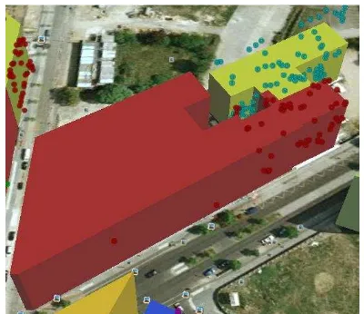
Finally, it is important to stress the variety of factors influencing the PS density. A good example for that is a trihedral reflection mechanism at a facade formed by the window sill, a part of the wall, and the frame of the window with just the right orientation to the sensors line of sight. If the window is always closed during the acquisition of just another image for the data stack, a PS is likely to be induced. However, if the window is opened once during an acquisition, the PS may be lost. In essence a lot of "random" processes decide if a reflection mechanism is persistent over the timeframe covered by the data stack. A quite nice example for such effect is shown in Figure 10. One part of the building complex shows a quite high PS density (around 3.6 PS per 1000m3) coloured in green. The other part exhibits a considerably lower density (0.5 PS per 1000m3) shown in red. A closer look at the actual PS distribution reveals, that PS could be found at the right part of the building only. The reason for that gets obvious in Figure 11, which shows an oblique view
aerial image (© MS-Bingmaps). A scaffold is visible in the left part suggesting ongoing construction works, which certainly leads to a loss of all PS at the particular building part.
5. CONCLUSION
A work flow aiming at the fusion of PS point clouds with building outlines for the purpose of determining the PS density per building has been demonstrated. The procedure consists of two steps namely alignment of PS and map data and assignment of PS to buildings. A simple Iterative Closest Point algorithm turned out to be sufficient for the alignment. The straightforward assignment of PS to the closest buildings could be improved to enhance the algorithms accuracy in dense built up areas. In some cases it might be reasonable to check if a set of regular shapes (e.g. planes obtained by extruding the polygon edges) can be fitted to the PS assigned to one building. However, this is quite difficult due to the quite inaccurate geocoding of PS and would definitely fail in case of complex roof structures leading to an irregular point distribution. The map of PS densities is a good tool to get an overview which buildings exhibit a sufficient PS coverage for monitoring purposes. However, it does not account for the PS distribution at the building. For that a matching of the PS to the polygon edges is thinkable. The main problem at that is to distinguish facade and roof PS which would ultimately boil down to the use of a distance threshold.
A better way would be to use a 3D city model and match the PS to bounding faces.
Finally, the PS density at buildings is quite heterogeneous for Figure 8. Oblique aerial image of test area "a". The different
facade structures, leading to quite heterogeneous PS densities, are clearly visible.
Figure 9. PS density in test area b. The building parts marked by the black rectangles show a quite low PS density because just
their roofs are visible to the sensor.
Figure 10. PS density for test area c. One part of the building (red) shows a very low PS density, while the other part shows
a quite good coverage (green). The reason for that are construction works.
Figure 11. Oblique view aerial image of test area c. The scaffold at the left part of the visible facade indicates construction works and explains the low PS density for this part of the building.
the investigated scene. While facade and roof structure as well as geometric configuration play the major role, a lot of factors may determine a buildings coverage.
6. REFERENCES
Auer, S., Gernhardt, S., Bamler, R., 2011. Investigations on the nature of Persistent Scatterers based on simulation methods. Proc. of the Urban Remote Sensing Even (JURSE) 2011, Munich, 11-13 April, pp. 61-64 (on CD-ROM).
Besl, P. J., McKay, N. D., 1992. A Method for Registration of 3-D Shapes. IEEE Transactions on Pattern Analysis and Machine Vision 14(2), pp. 239-256.
Ferretti, A., Prati, C., Rocca, F., 2000. Nonlinear Subsidance Rate Estimation Using Permanent Scatterers in Differential SAR Interferometry. IEEE Transactions on Geoscience and Remote Sensing 38(5), pp. 2202-2212.
Hooper, A., 2006. Persistent Scatterer Radar Interferometry for Crustal Deformation Studies and Modeling of Volcanic Deformation. Ph.D. dissertation, Stanford University.
Gernhardt, S., Adam, N., Eineder, M., Bamler, R., 2010. Potentials of very high resolution SAR for persistent scatterer interferometry in urban areas. Annals of GIS 16 (2), pp. 103-111.
Gernhardt, S., Cong, X., Eineder, M., Hinz, S., Bamler, R., 2011. Geometrical fusion of multitrack ps point clouds. IEEE Geoscience and Remote Sensing Letters 9(1), pp. 38-42.
Liu, G., Buckley, S. M., Ding, X., Cheng, Q. , Luo, X., 2009. Estimating Spatiotemporal Ground Deformation With Improved Permanent Scatterer Radar Interferometry”, IEEE Transactions on Geoscience and Remote Sensing. 47 (8), pp. 2762-2772.