TE
AM
Other Titles in the McGraw-Hill Demystified Series
Algebra Demystifiedby Rhonda Huettenmueller
Astronomy Demystifiedby Stan Gibilisco
STEVEN G. KRANTZ
McGRAW-HILL
Copyright © 2003 by The McGraw-Hill Companies, Inc.. All rights reserved. Manufactured in the United States of America. Except as permitted under the United States Copyright Act of 1976, no part of this publication may be reproduced or distributed in any form or by any means, or stored in a database or retrieval system, without the prior written permission of the publisher.
0-07-141211-5
The material in this eBook also appears in the print version of this title: 0-07-139308-0.
All trademarks are trademarks of their respective owners. Rather than put a trademark symbol after every occurrence of a trade-marked name, we use names in an editorial fashion only, and to the benefit of the trademark owner, with no intention of infringe-ment of the trademark. Where such designations appear in this book, they have been printed with initial caps.
McGraw-Hill eBooks are available at special quantity discounts to use as premiums and sales promotions, or for use in corporate training programs. For more information, please contact George Hoare, Special Sales, at [email protected] or (212) 904-4069.
TERMS OF USE
This is a copyrighted work and The McGraw-Hill Companies, Inc. (“McGraw-Hill”) and its licensors reserve all rights in and to the work. Use of this work is subject to these terms. Except as permitted under the Copyright Act of 1976 and the right to store and retrieve one copy of the work, you may not decompile, disassemble, reverse engineer, reproduce, modify, create derivative works based upon, transmit, distribute, disseminate, sell, publish or sublicense the work or any part of it without McGraw-Hill’s prior con-sent. You may use the work for your own noncommercial and personal use; any other use of the work is strictly prohibited. Your right to use the work may be terminated if you fail to comply with these terms.
THE WORK IS PROVIDED “AS IS”. McGRAW-HILL AND ITS LICENSORS MAKE NO GUARANTEES OR WARRANTIES AS TO THE ACCURACY, ADEQUACY OR COMPLETENESS OF OR RESULTS TO BE OBTAINED FROM USING THE WORK, INCLUDING ANY INFORMATION THAT CAN BE ACCESSED THROUGH THE WORK VIA HYPERLINK OR OTHERWISE, AND EXPRESSLY DISCLAIM ANY WARRANTY, EXPRESS OR IMPLIED, INCLUDING BUT NOT LIMITED TO IMPLIED WARRANTIES OF MERCHANTABILITY OR FITNESS FOR A PARTICULAR PURPOSE. McGraw-Hill and its licensors do not warrant or guarantee that the functions contained in the work will meet your requirements or that its operation will be uninterrupted or error free. Neither McGraw-Hill nor its licensors shall be liable to you or anyone else for any inaccuracy, error or omission, regardless of cause, in the work or for any damages resulting therefrom. McGraw-Hill has no responsibility for the con-tent of any information accessed through the work. Under no circumstances shall McGraw-Hill and/or its licensors be liable for any indirect, incidental, special, punitive, consequential or similar damages that result from the use of or inability to use the work, even if any of them has been advised of the possibility of such damages. This limitation of liability shall apply to any claim or cause what-soever whether such claim or cause arises in contract, tort or otherwise.
Preface
xi
CHAPTER 1
Basics
1
1.0 Introductory Remarks 1
1.1 Number Systems 1
1.2 Coordinates in One Dimension 3
1.3 Coordinates in Two Dimensions 5
1.4 The Slope of a Line in the Plane 8
1.5 The Equation of a Line 13
1.6 Loci in the Plane 15
1.7 Trigonometry 19
1.8 Sets and Functions 30
1.8.1 Examples of Functions of a Real Variable 31
1.8.2 Graphs of Functions 33
1.8.3 Plotting the Graph of a Function 35
1.8.4 Composition of Functions 40
1.8.5 The Inverse of a Function 42
1.9 A Few Words About Logarithms and Exponentials 49
CHAPTER 2
Foundations of Calculus
57
2.1 Limits 57
2.1.1 One-Sided Limits 60
2.2 Properties of Limits 61
2.3 Continuity 64
2.4 The Derivative 66
2.5 Rules for Calculating Derivatives 71
2.5.1 The Derivative of an Inverse 76
2.6 The Derivative as a Rate of Change 76
Contents
viii
CHAPTER 3
Applications of the Derivative
81
3.1 Graphing of Functions 81
3.2 Maximum/Minimum Problems 86
3.3 Related Rates 91
3.4 Falling Bodies 94
CHAPTER 4
The Integral
99
4.0 Introduction 99
4.1 Antiderivatives and Indefinite Integrals 99
4.1.1 The Concept of Antiderivative 99
4.1.2 The Indefinite Integral 100
4.2 Area 103
4.3 Signed Area 111
4.4 The Area Between Two Curves 116
4.5 Rules of Integration 120
4.5.1 Linear Properties 120
4.5.2 Additivity 120
CHAPTER 5
Indeterminate Forms
123
5.1 l’Hôpital’s Rule 123
5.1.1 Introduction 123
5.1.2 l’Hôpital’s Rule 124
5.2 Other Indeterminate Forms 128
5.2.1 Introduction 128
5.2.2 Writing a Product as a Quotient 128
5.2.3 The Use of the Logarithm 128
5.2.4 Putting Terms Over a Common Denominator 130
5.2.5 Other Algebraic Manipulations 131
5.3 Improper Integrals: A First Look 132
5.3.1 Introduction 132
5.3.2 Integrals with Infinite Integrands 133
5.3.3 An Application to Area 139
5.4 More on Improper Integrals 140
5.4.1 Introduction 140
5.4.2 The Integral on an Infinite Interval 141
6.2.2 Calculus Properties of the Exponential 156
6.2.3 The Numbere 158
6.3 Exponentials with Arbitrary Bases 160
6.3.1 Arbitrary Powers 160
6.3.2 Logarithms with Arbitrary Bases 163
6.4 Calculus with Logs and Exponentials to Arbitrary Bases 166
6.4.1 Differentiation and Integration of logaxandax 166
6.4.2 Graphing of Logarithmic and Exponential
Functions 168
6.4.3 Logarithmic Differentiation 170
6.5 Exponential Growth and Decay 172
6.5.1 A Differential Equation 173
6.5.2 Bacterial Growth 174
6.5.3 Radioactive Decay 176
6.5.4 Compound Interest 178
6.6 Inverse Trigonometric Functions 180
6.6.1 Introductory Remarks 180
6.6.2 Inverse Sine and Cosine 180
6.6.3 The Inverse Tangent Function 185
6.6.4 Integrals in Which Inverse Trigonometric Functions
Arise 187
6.6.5 Other Inverse Trigonometric Functions 189
6.6.6 An Example Involving Inverse Trigonometric
Functions 193
CHAPTER 7
Methods of Integration
197
7.1 Integration by Parts 197
7.2 Partial Fractions 202
7.2.1 Introductory Remarks 202
7.2.2 Products of Linear Factors 203
Contents
x
7.3 Substitution 207
7.4 Integrals of Trigonometric Expressions 210
CHAPTER 8
Applications of the Integral
217
8.1 Volumes by Slicing 217
8.1.0 Introduction 217
8.1.1 The Basic Strategy 217
8.1.2 Examples 219
8.2 Volumes of Solids of Revolution 224
8.2.0 Introduction 224
8.2.1 The Method of Washers 225
8.2.2 The Method of Cylindrical Shells 228
8.2.3 Different Axes 231
8.3 Work 233
8.4 Averages 237
8.5 Arc Length and Surface Area 240
8.5.1 Arc Length 240
8.5.2 Surface Area 243
8.6 Hydrostatic Pressure 247
8.7 Numerical Methods of Integration 252
8.7.1 The Trapezoid Rule 253
8.7.2 Simpson’s Rule 256
Bibliography
263
Solutions to Exercises
265
Final Exam
313
Index
339
TE
AM
arguably the cornerstone of modern science. Any well-educated person should at least be acquainted with the ideas of calculus, and a scientifically literate person must know calculus solidly.
Calculus has two main aspects: differential calculus and integral calculus. Differential calculus concerns itself with rates of change. Various types of change, both mathematical and physical, are described by a mathematical quantity called thederivative. Integral calculus is concerned with a generalized type of addition, or amalgamation, of quantities. Many kinds of summation, both mathematical and physical, are described by a mathematical quantity called theintegral.
What makes the subject of calculus truly powerful and seminal is the Funda-mental Theorem of Calculus, which shows how an integral may be calculated by using the theory of the derivative. The Fundamental Theorem enables a number of important conceptual breakthroughs and calculational techniques. It makes the subject of differential equations possible (in the sense that it gives us ways tosolve
these equations).
Calculus Demystifiedexplains this panorama of ideas in a step-by-step and acces-sible manner. The author, a renowned teacher and expositor, has a strong sense of the level of the students who will read this book, their backgrounds and their strengths, and can present the material in accessible morsels that the student can study on his own. Well-chosen examples and cognate exercises will reinforce the ideas being presented. Frequent review, assessment, and application of the ideas will help students to retain and to internalize all the important concepts of calculus. We envision a book that will give the student a firm grounding in calculus. The student who has mastered this book will be able to go on to study physics, engineering, chemistry, computational biology, computer science, and other basic scientific areas that use calculus.
Calculus Demystified will be a valuable addition to the self-help literature. Written by an accomplished and experienced teacher (the author ofHow to Teach Mathematics), this book will aid the student who is working without a teacher.
Preface
xii
It will provide encouragement and reinforcement as needed, and diagnostic exer-cises will help the student to measure his or her progress. A comprehensive exam at the end of the book will help the student to assess his mastery of the subject, and will point to areas that require further work.
We expect this book to be the cornerstone of a series of elementary mathematics books of the same tenor and utility.
Steven G. Krantz
1.0
Introductory Remarks
Calculus is one of the most important parts of mathematics. It is fundamental to all of modern science. How could one part of mathematics be of such central impor-tance? It is because calculus gives us the tools to studyrates of changeandmotion. All analytical subjects, from biology to physics to chemistry to engineering to math-ematics, involve studying quantities that are growing or shrinking or moving—in other words, they arechanging. Astronomers study the motions of the planets, chemists study the interaction of substances, physicists study the interactions of physical objects. All of these involve change and motion.
In order to study calculus effectively, you must be familiar with cartesian geome-try, with trigonomegeome-try, and with functions. We will spend this first chapter reviewing the essential ideas. Some readers will study this chapter selectively, merely review-ing selected sections. Others will, for completeness, wish to review all the material. The main point is to get started on calculus (Chapter 2).
1.1
Number Systems
The number systems that we use in calculus are thenatural numbers, theintegers, therational numbers, and thereal numbers. Let us describe each of these:
• The natural numbers are the system of positive counting numbers 1, 2, 3, …. We denote the set of all natural numbers byN.
CHAPTER 1
Basics
2
• The integers are the positive and negative whole numbers and zero:
. . . ,−3,−2,−1, 0, 1, 2, 3,. . .. We denote the set of all integers byZ.
• The rational numbers are quotients of integers. Any number of the formp/q, withp, q ∈ Zand q = 0, is a rational number. We say thatp/q and r/s
represent thesame rational numberprecisely whenps=qr. Of course you know that in displayed mathematics we write fractions in this way:
1 2 +
2 3 =
7 6.
• The real numbers are the set of all decimals, both terminating and non-terminating. This set is rather sophisticated, and bears a little discussion. A decimal number of the form
x =3.16792 is actually a rational number, for it represents
x =3.16792= 316792 100000. A decimal number of the form
m=4.27519191919. . . ,
with a group of digits that repeats itself interminably, is also a rational number. To see this, notice that
100·m=427.519191919. . .
and therefore we may subtract:
100m=427.519191919. . . m= 4.275191919. . .
Subtracting, we see that
99m=423.244 or
m= 423244
99000.
So, as we asserted,mis a rational number or quotient of integers.
1.2
Coordinates in One Dimension
We envision the real numbers as laid out on a line, and we locate real numbers from left to right on this line. Ifa < bare real numbers thenawill lie to the left ofbon this line. See Fig. 1.1.
_ 3 _2 _1 0 1 2 3 4
a b
Fig. 1.1
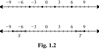
EXAMPLE 1.1
On a real number line, plot the numbers−4, −1, 2, 6. Also plot the sets
S= {x∈R: −8≤x <−5}andT = {t ∈R:7< t ≤9}. Label the plots.
SOLUTION
Figure 1.2 exhibits the indicated points and the two sets. These sets are called
half-open intervalsbecause each set includes one endpoint and not the other.
_ 9 _ 6 _ 3 0 3 6 9 _ 9 _ 6 _ 3 0 3 6 9
T S
Fig. 1.2
Math Note: The notation S = {x ∈ R: −8 ≤ x < −5} is calledset builder notation. It says thatSis the set of all numbersxsuch thatxis greater than or equal to−8 and less than 5. We will use set builder notation throughout the book.
If an interval contains both its endpoints, then it is called aclosed interval. If an interval omits both its endpoints, then it is called anopen interval. See Fig. 1.3.
open interval closed interval
CHAPTER 1
Basics
4
EXAMPLE 1.2
Find the set of points that satisfyx−2<4 and exhibit it on a number line.
SOLUTION
We solve the inequality to obtain x <6. The set of points satisfying this inequality is exhibited in Fig. 1.4.
_ 9 _ 6 _ 3 0 3 6 9
Fig. 1.4
EXAMPLE 1.3
Find the set of points that satisfy the condition
|x+3| ≤2 (*)
and exhibit it on a number line.
SOLUTION
In casex+3≥0 then|x+3| =x+3 and we may write condition(∗)as
x+3≤2 or
x≤ −1.
Combiningx+3≥0 andx ≤ −1 gives−3≤x ≤ −1.
On the other hand, ifx+3<0 then|x+3| = −(x+3). We may then write condition(∗)as
−(x+3)≤2 or
−5≤x.
Combiningx+3<0 and−5≤xgives−5≤x <−3.
We have found that our inequality|x+3| ≤2 is true precisely when either
−3≤x≤ −1 or−5≤x <−3. Putting these together yields−5≤x≤ −1. We display this set in Fig. 1.5.
_ 9 _ 6 _ 3 0 3 6 9
Fig. 1.5
You Try It: Solve the inequality|x−4|>1. Exhibit your answer on a number line.
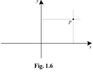
. The idea is best understood by way of some examples.
y
x P
Fig. 1.6
EXAMPLE 1.4
Plot the pointsP =(3,−2),Q=(−4,6),R=(2,5),S=(−5,−3).
SOLUTION
The first coordinate 3 of the pointP tells us that the point is located 3 units to therightof they-axis (because 3 ispositive). The second coordinate−2 of the pointP tells us that the point is located 2 unitsbelowthex-axis (because
−2 is negative). See Fig. 1.7.
The first coordinate−4 of the pointQtells us that the point is located 4 units to theleftof they-axis (because−4 isnegative). The second coordinate 6 of the pointQtells us that the point is located 6 unitsabovethex-axis (because 6 is positive). See Fig. 1.7.
The first coordinate 2 of the pointRtells us that the point is located 2 units to therightof they-axis (because 2 ispositive). The second coordinate 5 of the pointRtells us that the point is located 5 unitsabovethex-axis (because 5 is positive). See Fig. 1.7.
The first coordinate−5 of the pointStells us that the point is located 5 units to theleftof they-axis (because−5 isnegative). The second coordinate−3 of the pointStells us that the point is located 3 unitsbelowthex-axis (because
CHAPTER 1
Basics
6
y
4
1
x Q
S P
R
1 4
Fig. 1.7
EXAMPLE 1.5
Give the coordinatesof the pointsX, Y, Z, W exhibited in Fig. 1.8.
y
x
X
W
Z
Y
Fig. 1.8
SOLUTION
The pointXis 1 unit to the right of they-axis and 3 units below thex-axis. Therefore its coordinates are(1,−3).
EXAMPLE 1.6
Sketch the set of pointsℓ = {(x, y):y = 3}. Sketch the set of pointsk =
{(x, y):x = −4}.
SOLUTION
The setℓconsists of all points withy-coordinate equal to 3. This is the set of all points that lie 3 units above thex-axis. We exhibitℓin Fig. 1.9. It is a horizontal line.
l
Fig. 1.9
The setkconsists of all points withx-coordinate equal to−4. This is the set of all points that lie 4 units to the left of they-axis. We exhibitkin Fig. 1.10. It is a vertical line.
EXAMPLE 1.7
Sketch the set of pointsS= {(x, y):x >2}on a pair of coordinate axes.
SOLUTION
Notice that the set S contains all points with x-coordinate greater than 2. These will be all points to the right of the vertical line x = 2. That set is exhibited in Fig. 1.11.
You Try It: Sketch the set{(x, y):x+y <4}.
CHAPTER 1
Basics
8
k
Fig. 1.10
x y
Fig. 1.11
1.4
The Slope of a Line in the Plane
A line in the plane may rise gradually from left to right, or it may rise quite steeply from left to right (Fig. 1.13). Likewise, it could fall gradually from left to right, or it could fall quite steeply from left to right (Fig. 1.14). The number “slope” differentiates among these different rates of rise or fall.
Look at Fig. 1.15. We use the two points P = (p1, p2)and Q = (q1, q2)to calculate the slope. It is
m=q2−p2 q1−p1.
TE
AM
x 1
Fig. 1.12
y
x
Fig. 1.13
It turns out that, no matter which two points we may choose on a given line, this calculation will always give the same answer for slope.
EXAMPLE 1.8
Calculate the slope of the line in Fig. 1.16.
SOLUTION
We use the pointsP = (−1,0) and Q = (1,3)to calculate the slope of this line:
m= 3−0
1−(−1) =
CHAPTER 1
Basics
10
y
x
Fig. 1.14
y
x Q
P
Fig. 1.15
We could just as easily have used the pointsP = (−1,0)andR =(3,6)to calculate the slope:
m= 6−0
3−(−1) =
6 4 =
3 2.
x
Fig. 1.16
y
x R = (_ 2,10)
S = (_ 1,5)
T = (1,_ 5) 2 2 4 6 8 10
4 6
Fig. 1.17
EXAMPLE 1.9
Calculate the slope of the line in Fig. 1.17.
SOLUTION
We use the pointsR =(−2,10)andT =(1,−5)to calculate the slope of this line:
CHAPTER 1
Basics
12
We could just as easily have used the pointsS=(−1,5)andT =(1,−5):
m= 5−(−5)
−1−1 = −5.
In this example, the line falls 5 units for each 1 unit of left-to-right motion. The negativity of the slope indicates that the line is falling.
The concept of slope is undefined for a vertical line. Such a line will have any two points with the same x-coordinate, and calculation of slope would result in division by 0.
You Try It: What is the slope of the liney =2x+8?
You Try It: What is the slope of the line y = 5? What is the slope of the line
x=3?
Two lines are perpendicular precisely when their slopes are negative reciprocals. This makes sense: If one line has slope 5 and the other has slope −1/5 then we see that the first line rises 5 units for each unit of left-to-right motion while the second line falls 1 unit for each 5 units of left-to-right motion. So the lines must be perpendicular. See Fig. 1.18(a).
y
x
Fig. 1.18(a)
You Try It: Sketch the line that is perpendicular tox+2y=7 and passes through
(1,4).
Fig. 1.18(b)
1.5
The Equation of a Line
The equation of a line in the plane will describe—in compact form—all the points that lie on that line. We determine the equation of a given line by writing its slope in two different ways and then equating them. Some examples best illustrate the idea.
EXAMPLE 1.10
Determine the equation of the line with slope 3 that passes through the point
(2,1).
SOLUTION
Let(x, y)be a variable point on the line. Then we can use that variable point together with(2,1)to calculate the slope:
m= y−1 x−2.
On the other hand, we are given that the slope ism =3. We may equate the two expressions for slope to obtain
3= y−1
x−2. (∗)
This may be simplified toy=3x−5.
Math Note: The formy =3x−5 for the equation of a line is called the slope-intercept form. The slope is 3 and the line passes through(0,5)(itsy-intercept).
CHAPTER 1
Basics
14
You Try It: Write the equation of the line that passes through the point(−3,2)
and has slope 4.
EXAMPLE 1.11
Write the equation of the line passing through the points(−4,5)and(6,2).
SOLUTION
Let(x, y)be a variable point on the line. Using the points(x, y)and(−4,5), we may calculate the slope to be
m= y−5 x−(−4).
On the other hand, we may use the points(−4,5)and (6,2)to calculate the slope:
m= 2−5
6−(−4) =
−3 10. Equating the two expressions for slope, we find that
y−5
x+4 =
−3 10.
Simplifying this identity, we find that the equation of our line is
y−5= −3
10 ·(x+4).
You Try It: Find the equation of the line that passes through the points(2,−5)
and(−6,1).
In general, the line that passes through points(x0, y0)and(x1, y1)has equation
y−y0 x−x0 =
y1−y0 x1−x0.
This is called thetwo-point formof the equation of a line.
EXAMPLE 1.12
Find the line perpendicular toy = 3x−6 that passes through the point
(5,4).
SOLUTION
We know from the Math Note immediately after Example 1.10 that the given line has slope 3. Thus the line we seek (the perpendicular line) has slope−1/3. Using the point-slope form of a line, we may immediately write the equation of the line with slope−1/3 and passing through(5,4)as
y−4= −1
− 0
x−x0 =
1− 0
x1−x0.
This is the two-point form of a line.
You Try It: Find the line perpendicular to 2x +5y = 10 that passes through the point(1,1). Now find the line that is parallel to the given line and passes through(1,1).
1.6
Loci in the Plane
The most interesting sets of points to graph are collections of points that are defined by an equation. We call such a graph thelocusof the equation. We cannot give all the theory of loci here, but instead consider a few examples. See [SCH2] for more on this matter.
EXAMPLE 1.13
Sketch the graph of{(x, y):y =x2}.
SOLUTION
It is convenient to make a table of values:
x y =x2
−3 9
−2 4
−1 1
0 0
1 1
2 4
3 9
CHAPTER 1
Basics
16
y
x
Fig. 1.19
Fig. 1.20
EXAMPLE 1.14
Sketch the graph of the curve{(x, y):y=x3}.
SOLUTION
It is convenient to make a table of values:
x y=x3
−3 −27
−2 −8
−1 −1
0 0
1 1
2 8
3 27
x 3 6
Fig. 1.21
Fig. 1.22
You Try It: Sketch the graph of the locus|x| = |y|.
EXAMPLE 1.15
CHAPTER 1
Basics
18
SOLUTION
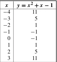
It is convenient to make a table of values:
x y=x2+x−1
−4 11
−3 5
−2 1
−1 −1
0 −1
1 1
2 5
3 11
We plot these points on a single set of axes (Fig. 1.23). Supposing that the curve we seek to draw is a smooth interpolation of these points (calculus will later show us that this supposition is correct), we find that our curve is as shown in Fig. 1.24. This is another example of a parabola.
y
x
Fig. 1.23
You Try It: Sketch the locusy2=x3+x+1 on a set of axes.
The reader unfamiliar with cartesian geometry and the theory of loci would do well to consult [SCH2].
TE
AM
Fig. 1.24
1.7
Trigonometry
Here we give a whirlwind review of basic ideas of trigonometry. The reader who needs a more extensive review should consult [SCH1].
When we first learn trigonometry, we do so by studying right triangles and measuring angles in degrees. Look at Fig. 1.25. In calculus, however, it is convenient to study trigonometry in a more general setting, and to measure angles in radians.
=
= measured in degrees
Fig. 1.25
CHAPTER 1
Basics
20
α
y
x
positive angle
Fig. 1.26
α
y
x
negative angle
Fig. 1.27
In degree measure, one full rotation about the unit circle is 360◦; in radian measure, one full rotation about the circle is just the circumference of the circle or 2π. Let us use the symbolθ to denote an angle. The principle of proportionality now tells us that
degree measure ofθ
360◦ =
radian measure ofθ
2π .
In other words
radian measure ofθ = π
180 ·(degree measure ofθ ) and
degree measure ofθ = 180
the angle subtends an arc of the unit circle corresponding to 1/12 of the full cir-cumference. Sinceπ/6>0, the angle represents a counterclockwise rotation. It is illustrated in Fig. 1.28.
p/6
x y
Fig. 1.28
The degree measure of this angle is
180
π · π
6 =30 ◦.
Math Note: In this book wealwaysuse radian measure for angles. (The reason is that it makes the formulas of calculus turn out to be simpler.) Thus, for example, if we refer to “the angle 2π/3” then it should be understood that this is an angle in radian measure. See Fig. 1.29.
Likewise, if we refer to the angle 3 it is also understood to be radian measure. We sketch this last angle by noting that 3 is approximately 0.477 of a full rotation 2π—refer to Fig. 1.30.
CHAPTER 1
Basics
22
y
x 2F/3
Fig. 1.29
y
x 3
Fig. 1.30
EXAMPLE 1.17
Several anglesare sketched in Fig. 1.31, and both their radian and degree measures given.
Ifθ is an angle, let(x, y)be the coordinates of the terminal point of the corre-sponding radius (called theterminal radius) on the unit circle. We callP =(x, y)
theterminal pointcorresponding toθ. Look at Fig. 1.32. The numberyis called the
sineofθ and is written sinθ. The numberxis called thecosineofθ and is written cosθ.
Since (cosθ,sinθ )are coordinates of a point on the unit circle, the following two fundamental properties are immediate:
(1) For any numberθ,
_ 3p/4 = _135°
_p = _180° x
Fig. 1.31
y
x unit circle P = (x, y)
G
cos G sin G
Fig. 1.32
(2) For any numberθ,
−1≤cosθ ≤1 and −1≤sinθ ≤1.
Math Note: It is common to write sin2θ to mean (sinθ )2 and cos2θ to mean
(cosθ )2.
EXAMPLE 1.18
CHAPTER 1
Basics
24
SOLUTION
We sketch the terminal radius and associated triangle (see Fig. 1.33). This is a 30–60–90 triangle whose sides have ratios 1:√3:2. Thus
1
x =2 or x=
1 2. Likewise,
y x =
√
3 or y =√3x =
√
3 2 . It follows that
sinπ 3 =
√
3 2 and
cosπ 3 =
1 2.
unit circle
y
x
√3
2
1 2
F/3
Fig. 1.33
You Try It: The cosine of a certain angle is 2/3. The angle lies in the fourth quadrant. What is the sine of the angle?
Math Note: Notice that ifθis an angle thenθ andθ+2πhave the same terminal radius and the same terminal point (for adding 2πjust adds one more trip around the circle—look at Fig. 1.34).
As a result,
G
cosG
unit circle
x
Fig. 1.34
and
cosθ =y =cos(θ +2π ).
We say that the sine and cosine functions have period 2π: the functions repeat themselves every 2πunits.
In practice, when we calculate the trigonometric functions of an angle θ, we reduce it by multiples of 2π so that we can consider an equivalent angleθ′, called theassociated principal angle,satisfying 0≤θ′ <2π. For instance,
15π/2 has associated principal angle 3π/2 (since 15π/2−3π/2=3·2π )
and
−10π/3 has associated principal angle
2π/3 (since −10π/3−2π/3= −12π/3= −2·2π ).
You Try It: What are the principal angles associated with 7π, 11π/2, 8π/3,
−14π/5,−16π/7?
What does the concept of angle and sine and cosine that we have presented here have to do with the classical notion using triangles? Notice that any angleθ such that 0 ≤ θ < π/2 has associated to it a right triangle in the first quadrant, with vertex on the unit circle, such that the base is the segment connecting(0,0)to(x,0)
CHAPTER 1
Basics
26
unit circle adjacent side opposite side y x (x, y)G G
Fig. 1.35
Then
sinθ =y = y
1 =
opposite side of triangle hypotenuse
and
cosθ =x= x
1 =
adjacent side of triangle hypotenuse .
Thus, for anglesθbetween 0 andπ/2, the new definition of sine and cosine using the unit circle is clearly equivalent to the classical definition using adjacent and opposite sides and the hypotenuse. For other anglesθ, the classical approach is to reduce to this special case by subtracting multiples ofπ/2. Our approach using the unit circle is considerably clearer because it makes the signatures of sine and cosine obvious.
Besides sine and cosine, there are four other trigonometric functions:
tanθ = y x =
sinθ
cosθ
cotθ = x y =
cosθ
sinθ
secθ = 1 x =
1 cosθ
cscθ = 1 y =
1 sinθ.
Whereas sine and cosine have domain the entire real line, we notice that tanθ and secθ are undefined at odd multiples ofπ/2 (because cosine will vanish there) and cotθ and cscθ are undefined at even multiples ofπ/2 (because sine will vanish there). The graphs of the six trigonometric functions are shown in Fig. 1.36.
EXAMPLE 1.19
1 1
Fig. 1.36(a) Graphs ofy=sinxandy =cosx.
_ 6
_ 30 _ 20 _ 10 10 20 30
_ 4 _ 2 4 6 _ 6
_ 30 _ 20 _ 10 10 20 30
_ 4 _ 2 2 4 6 2
Fig. 1.36(b) Graphs ofy=tanxandy=cotx.
_ 6
_ 4 _ 2 2 4 6 15
10
5
_ 5 _10 _15
_ 6 _ 4 _ 2
2
4 6 15
10
5
_ 5 _10 _15
Fig. 1.36(c) Graphs ofy=secxandy=cscx.
SOLUTION
CHAPTER 1
Basics
28
1
√2
1
√2
unit circle y
x 11F/4
Fig. 1.37
Thereforex = −1/√2 andy=1/√2. It follows that sinθ =y = √1
2
cosθ =x = −√1
2
tanθ = y x = −1
cotθ = x y = −1
secθ = 1 x = −
√
2
cscθ = 1 y =
√
2.
Similar calculations allow us to complete the following table for the values of the trigonometric functions at the principal angles which are multiples ofπ/6 orπ/4.
TE
AM
2π/3 3/2 −1/2 − 3 −1/ 3 −2 2/ 3
3π/4 √2/2 −√2/2 −1 −1 −√2 √2
5π/6 1/2 −√3/2 −1/√3 −√3 −2/√3 2
π 0 −1 0 undef −1 undef
7π/6 −1/2 −√3/2 1/√3 √3 −2/√3 −2
5π/4 −√2/2 −√2/2 1 1 −√2 −√2
4π/3 −√3/2 −1/2 √3 1/√3 −2 −2/√3
3π/2 −1 0 undef 0 undef −1
5π/3 −√3/2 1/2 −√3 −1/√3 2 −2/√3
7π/4 −√2/2 √2/2 −1 −1 √2 −√2
11π/6 −1/2 √3/2 −1/√3 −√3 2/√3 −2 Besides properties (1) and (2) above, there are certain identities which are fundamental to our study of the trigonometric functions. Here are the principal ones:
(3) tan2θ +1=sec2θ (4) cot2θ +1=csc2θ
(5) sin(θ+ψ )=sinθcosψ+cosθsinψ (6) cos(θ +ψ )=cosθcosψ−sinθsinψ (7) sin(2θ )=2 sinθcosθ
(8) cos(2θ )=cos2θ−sin2θ (9) sin(−θ )= −sinθ (10) cos(−θ )=cosθ (11) sin2θ = 1−cos 2θ
2
(12) cos2θ = 1+cos 2θ
2
EXAMPLE 1.20
CHAPTER 1
Basics
30
SOLUTION
We have
tan2θ+1= sin 2θ cos2θ +1
= sin
2θ cos2θ +
cos2θ
cos2θ
= sin
2θ
+cos2θ
cos2θ
= cos12
θ
(where we have used Property (1))
=sec2θ.
You Try It: Use identities (11) and (12) to calculate cos(π/12)and sin(π/12).
1.8
Sets andFunctions
We have seen sets and functions throughout this review chapter, but it is well to bring out some of the ideas explicitly.
Asetis a collection of objects. We denote a set with a capital roman letter, such asSorT orU. IfSis a set andsis an object in that set then we writes ∈S and we say thatsis an element ofS. IfSandT are sets then the collection of elements common to the two sets is called theintersectionofSandT and is writtenS∩T. The set of elements that are inSor inT or in both is called theunionofSandT
and is writtenS∪T.
Afunctionfrom a setS to a setT is a rule that assigns to each element ofS a unique element ofT. We writef :S →T.
EXAMPLE 1.21
Let Sbe the set of all people who are alive at noon on October 10, 2004 and T the set of all real numbers. Letf be the rule that assigns to each person hisor her weight in poundsat precisely noon on October 10, 2004. Discuss whetherf :S→T isa function.
SOLUTION
EXAMPLE 1.23
LetS be the set of all people andT be the set of all strings of letters not exceeding 1500 characters (including blank spaces). Letf be the rule that assigns to each person his or her legal name. (Some people have rather long names; according to theGuinness Book of World Records, the longest has1063 letters.) Determine whetherf :S→T isa function.
SOLUTION
Thisf is a function because every person has one and only one legal name. Notice that several people may have the same name (such as “Jack Armstrong”), but that is allowed in the definition of function.
You Try It: Letf be the rule that assigns to each real number its cube root. Is this a function?
In calculus, the setS (called thedomainof the function) and the setT (called therangeof the function) will usually be sets of numbers; in fact they will often consist of one or more intervals inR. The rulef will usually be given by one or several formulas. Many times the domain and range will not be given explicitly. These ideas will be illustrated in the examples below.
You Try It: Consider the rule that assigns to each real number its absolute value. Is this a function? Why or why not? If it is a function, then what are its domain and range?
1.8.1
EXAMPLES OF FUNCTIONS OF A REAL
VARIABLE
EXAMPLE 1.24
LetS =R,T = R, and letf (x)= x2. Thisismathematical shorthand for the rule “assign to eachx ∈ Sitssquare.” Determine whetherf :R→R
isa function.
SOLUTION
CHAPTER 1
Basics
32
Math Note: Notice that, in the definition of function, there is some imprecision in the definition ofT. For instance, in Example 1.24, we could have letT = [0,∞)
orT =(−6,∞)with no significant change in the function. In the example of the “name” function (Example 1.23), we could have letT be all strings of letters not exceeding 5000 characters in length. Or we could have made it all strings without regard to length. Likewise, in any of the examples we could make the setSsmaller and the function would still make sense.
It is frequently convenient not to describeSandT explicitly.
EXAMPLE 1.25
Letf (x) = +√1−x2. Determine a domain and range forf which make
f a function.
SOLUTION
Notice thatf makes sense forx ∈ [−1,1](we may not take the square root of a negative number, so we cannot allowx >1 orx <−1). If we understand
f to have domain[−1,1]and rangeR, thenf : [−1,1] →Ris a function.
Math Note: When a function is given by a formula, as in Example 1.25, with no statement about the domain, then the domain is understood to be the set of allxfor which the formula makes sense.
You Try It: Let
g(x)= x x2+4x+3. What are the domain and range of this function?
EXAMPLE 1.26
Let
f (x)=
−3 ifx≤1 2x2 ifx >1
Determine whetherf isa function.
SOLUTION
Notice thatf unambiguously assigns toeachreal number another real num-ber. The rule is given in two pieces, but it is still a valid rule. Therefore it is a function with domain equal to Rand range equal toR. It is also perfectly correct to take the range to be(−4,∞), for example, sincefonly takes values in this set.
Letf (x)= ± x. Discuss whetherf isa function.
SOLUTION
Thisf can only make sense forx ≥ 0. But even thenf isnota function since it is ambiguous. For instance, it assigns tox = 1 both the numbers 1 and−1.
1.8.2
GRAPHS OF FUNCTIONS
It is useful to be able to draw pictures which represent functions. These pictures, orgraphs, are a device for helping us to think about functions. In this book we will only graph functions whose domains and ranges are subsets of the real numbers.
We graph functions in thex-yplane. The elements of the domain of a function are thought of as points of thex-axis. The values of a function are measured on the
y-axis. The graph offassociates toxthe uniqueyvalue that the functionf assigns tox. In other words, a point(x, y)lies on the graph off if and only ify=f (x).
EXAMPLE 1.28
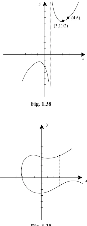
Let f (x) = (x2 +2)/(x−1). Determine whether there are pointsof the graph off corresponding tox =3,4, and 1.
SOLUTION
The y value corresponding to x = 3 isy = f (3) = 11/2. Therefore the point(3,11/2)lies on the graph off. Similarly,f (4)=6 so that(4,6)lies on the graph. However,f is undefined atx=1, so there is no point on the graph withx coordinate 1. The sketch in Fig. 1.38 was obtained by plotting several points.
Math Note: Notice that for eachxin the domain of the function there isone and only onepoint on the graph—namely the unique point withyvalue equal tof (x). Ifx is not in the domain off, then there is no point on the graph that corresponds tox.
EXAMPLE 1.29
CHAPTER 1
Basics
34
Fig. 1.38
Fig. 1.39
SOLUTION
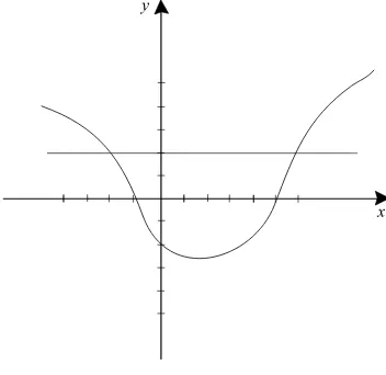
Observe that, corresponding tox =3, for instance, there are twoy values on the curve. Therefore the curve cannot be the graph of a function.
You Try It: Graph the functiony=x+ |x|.
EXAMPLE 1.30
Fig. 1.40
SOLUTION
Notice that each x in the domain has just oney value corresponding to it. Thus, even though we cannot give a formula for the function, the curve is the graph of a function. The domain of this function is(−∞,3)∪(5,7).
Math Note: A nice, geometrical way to think about the condition that eachxin the domain has corresponding to it precisely oneyvalue is this:
If every vertical line drawn through a curve intersects that curve just once, then the curve isthe graph of a function.
You Try It: Use the vertical line test to determine whether the locusx2+y2=1 is the graph of a function.
1.8.3
PLOTTING THE GRAPH OF A FUNCTION
Until we learn some more sophisticated techniques, the basic method that we shall use for graphing functions is to plot points and then to connect them in a plausible manner.
EXAMPLE 1.31
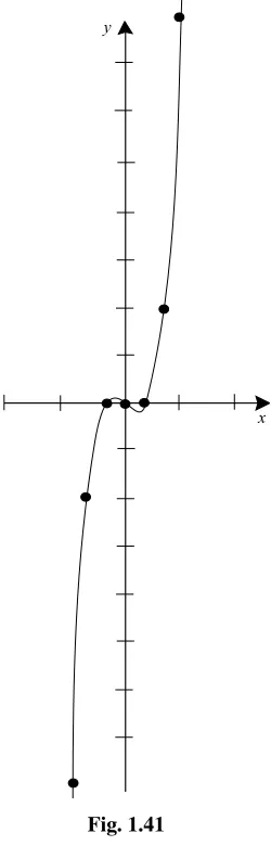
Sketch the graph off (x)=x3−x.
SOLUTION
CHAPTER 1
Basics
36
x y=x3−x
−3 −24
−2 −6
−1 0
0 0
1 0
2 6
3 24
We plot these points on a pair of axes and connect them in a reasonable way (Fig. 1.41). Notice that the domain off is all ofR, so we extend the graph to the edges of the picture.
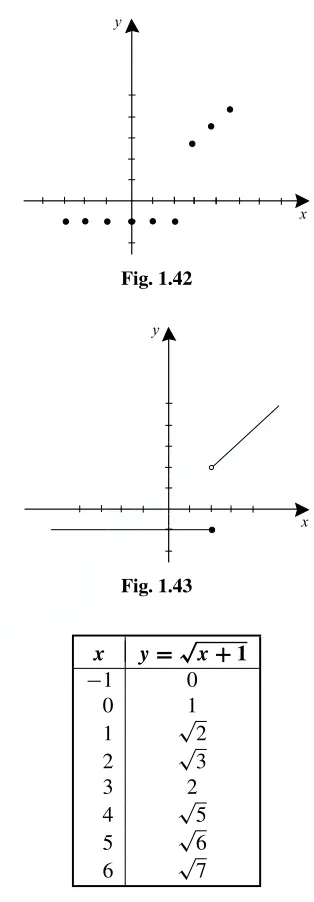
EXAMPLE 1.32
Sketch the graph of
f (x)=
−1 ifx ≤2
x ifx >2
SOLUTION
We again start with a table of values.
x y=f (x)
−3 −1
−2 −1
−1 −1
0 −1
1 −1
2 −1
3 3
4 4
5 5
We plot these on a pair of axes (Fig. 1.42).
Since the definition of the function changes atx =2, we would be mistaken to connect these dots blindly. First notice that, for x ≤ 2, the function is identically constant. Its graph is a horizontal line. Forx >2, the function is a line of slope 1. Now we can sketch the graph accurately (Fig. 1.43).
Fig. 1.41
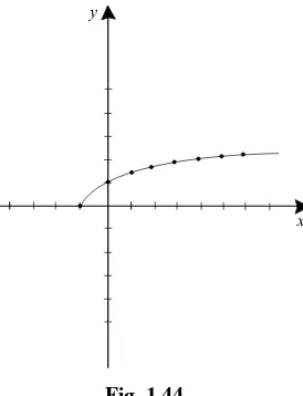
EXAMPLE 1.33
Sketch the graph off (x)=√x+1 .
SOLUTION
CHAPTER 1
Basics
38
y
x
Fig. 1.42
y
x
Fig. 1.43
x y=√x+1
−1 0
0 1
1 √2
2 √3
3 2
4 √5
5 √6
6 √7
Connecting the points in a plausible way gives a sketch for the graph off
(Fig. 1.44).
EXAMPLE 1.34
Sketch the graph ofx=y2.
TE
AM
Fig. 1.44
SOLUTION
The sketch in Fig. 1.45 is obtained by plotting points. This curve isnotthe graph of a function.
Fig. 1.45
A curve that is the plot of an equation but which isnot necessarilythe graph of a function is sometimes called thelocusof the equation. When the curveis
the graph of a function we usually emphasize this fact by writing the equation in the formy =f (x).
CHAPTER 1
Basics
40
1.8.4
COMPOSITION OF FUNCTIONS
Suppose thatfandgare functions and that the domain ofgcontains the range off. This means that ifxis in the domain off thenf (x)makes sense but alsogmay be applied tof (x)(Fig. 1.46). The result of these two operations, one following the other, is calledgcomposedwithf or thecompositionofgwithf. We write
(g◦f )(x)=g(f (x)).
x f(x) g(f(x))
Fig. 1.46
EXAMPLE 1.35
Letf (x)=x2−1 andg(x)=3x+4. Calculateg◦f.
SOLUTION
We have
(g◦f )(x)=g(f (x))=g(x2−1). (∗) Notice that we have started to workinside the parentheses: the first step was to substitute the definition off, namelyx2−1, into our equation.
Now the definition ofgsays that we takegofanyargument by multiplying that argument by 3 and then adding 4. In the present case we are applyinggto
x2−1. Therefore the right side of equation(∗)equals 3·(x2−1)+4.
This easily simplifies to 3x2+1. In conclusion,
g◦f (x)=3x2+1. EXAMPLE 1.36
Letf (t)=(t2−2)/(t+1)andg(t)=2t+1. Calculateg◦f andf ◦g.
SOLUTION
We calculate that
(g◦f )(t )=g(f (t ))=g
t2−2
t+1
= 2t +t−3
t+1 .
One of the main points of this example is to see thatf ◦gis different from
g◦f. We computef ◦g:
(f ◦g)(t )=f (g(t ))
=f (2t+1)
=(2t+1)
2
−2
(2t+1)+1
=4t
2
+4t−1 2t+2 . Sof ◦gandg◦f are different functions.
You Try It: Letf (x)= |x|andg(x)=√x/x. Calculatef ◦g(x)andg◦f (x). We say a few words aboutrecognizingcompositions of functions.
EXAMPLE 1.37
How can we write the functionk(x)=(2x+3)2asthe composition of two functionsgandf?
SOLUTION
Notice that the function k can be thought of as two operations applied in sequence. First we double and add three, then we square. Thus definef (x)=
2x+3 andg(x)=x2. Thenk(x)=(g◦f )(x). We can also compose three (or more) functions: Define
(h◦g◦f )(x)=h(g(f (x))). EXAMPLE 1.38
CHAPTER 1
Basics
42
SOLUTION
First we double, then we add 3, then we square. So letf (x)=2x,g(x)= x+3,h(x)=x2. Thenk(x)=(h◦g◦f )(x).
EXAMPLE 1.39
Write the function
r(t)= 2 t2+3 asthe composition of two functions.
SOLUTION
First we squaretand add 3, then we divide 2 by the quantity just obtained.As a result, we definef (t )=t2+3 andg(t )=2/t. It follows thatr(t )=(g◦f )(t ).
You Try It: Express the functiong(x) = 3/(x2+5)as the composition of two functions. Can you express it as the composition of three functions?
1.8.5
THE INVERSE OF A FUNCTION
Letf be the function which assigns to each working adult American his or her Social Security Number (a 9-digit string of integers). Letgbe the function which assigns to each working adult American his or her age in years (an integer between 0 and 150). Both functions have the same domain, and both take values in the non-negative integers. But there is a fundamental difference betweenf andg. If you are given a Social Security number, then you can determine the person to whom it belongs. There will be one and only one person with that number. But if you are given a number between 0 and 150, then there will probably be millions of people with that age. Youcannotidentify a person by his/her age. In summary, if you know
g(x)then you generallycannotdetermine whatxis. But if you knowf (x)then you
candetermine what (or who)xis. This leads to the main idea of this subsection. Letf : S → T be a function. We say thatf has an inverse (is invertible) if there is a functionf−1 : T → S such that (f ◦f−1)(t ) = t for allt ∈ T and
(f−1◦f )(s)=sfor alls ∈S. Notice that the symbolf−1denotes a new function which we call theinverseoff.
Basic Rule forFinding Inverses To find the inverse of a functionf, we solve the equation
(f ◦f−1)(t )=t
for the functionf−1(t ).
EXAMPLE 1.40
3·f−1(t )=t
or
f−1(t )= t
3. Thusf−1(t )=t /3.
EXAMPLE 1.41
Letf :R→Rbe defined byf (s)=3s5. Findf−1.
SOLUTION
We solve
(f ◦f−1)(t )=t
or
f (f−1(t ))=t
or
3[f−1(t )]5=t
or
[f−1(t )]5= t
3 or
f−1(t )=
t
3
1/5
.
You Try It: Find the inverse of the functiong(x)=√3x
−5.
It is important to understand that some functions donothave inverses.
EXAMPLE 1.42
CHAPTER 1
Basics
44
SOLUTION
Using the Basic Rule, we attempt to solve
(f ◦f−1)(t )=t.
Writing this out, we have
[f−1(t )]2 =t.
But now there is a problem: we cannot solve this equation uniquely forf−1(t ). We do not know whetherf−1(t )= +√torf−1(t )= −√t. Thusf−1is not a well defined function. Thereforef is not invertible andf−1does not exist.
Math Note: There is a simple device which often enables us to obtain an inverse— even in situations like Example 1.42. We change the domain of the function. This idea is illustrated in the next example.
EXAMPLE 1.43
Definef : {s :s ≥0} → {t :t ≥0}by the formulaf (s)=s2. Findf−1.
SOLUTION
We attempt to solve
(f◦f−1)(t )=t.
Writing this out, we have
f (f−1(t ))=t
or
[f−1(t )]2 =t.
This looks like the same situation we had in Example 1.42. But in fact things have improved. Now weknow thatf−1(t )must be+√t, because f−1must have rangeS = {s :s ≥0}. Thusf−1 : {t :t ≥0} → {s :s ≥0}is given by
f−1(t )= +√t.
You Try It: The equationy=x2+3xdoes not describe the graph of an invertible function. Find a way to restrict the domain so that it is invertible.
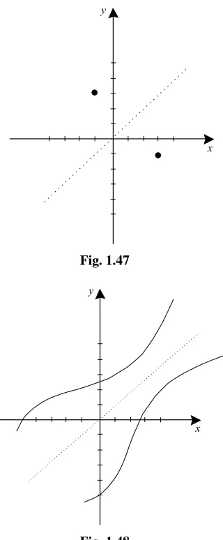
Now we consider the graph of the inverse function. Suppose that f : S → T
is invertible and that (s, t ) is a point on the graph of f. Thent = f (s) hence
s = f−1(t ) so that (t, s) is on the graph of f−1. The geometrical connection between the points(s, t )and(t, s)is exhibited in Fig. 1.47: they are reflections of each other in the liney =x. We have discovered the following important principle:
x
Fig. 1.47
y
x
Fig. 1.48
EXAMPLE 1.44
Sketch the graph of the inverse of the functionf whose graph is shown in Fig. 1.49.
SOLUTION
CHAPTER 1
Basics
46
Fig. 1.49
Fig. 1.50
You Try It: Sketchf (x)=x3+xand its inverse.
Another useful fact is this: Since an invertible function must be one-to-one, two differentx values cannot correspond to (that is, be “sent by the function to”) the sameyvalue. Looking at Figs. 1.51 and 1.52, we see that this means
In order forf to be invertible, no horizontal line can intersect the graph off more than once.
Fig. 1.52
EXAMPLE 1.45
Look at Figs. 1.53 and 1.55. Are the functionswhose graphsare shown in parts(a)and(b)of each figure invertible?
Fig. 1.53
SOLUTION
Graphs (a) and (b) in Fig. 1.53 are the graphs of invertible functions since no horizontal line intersects each graph more than once. Of course we must choose the domain and range appropriately. For (a) we takeS = [−4,4]and
CHAPTER 1
Basics
48
in Fig. 1.54 are the graphs of the inverse functions corresponding to (a) and (b) of Fig. 1.53 respectively. They are obtained by reflection in the liney =x.
Fig. 1.54
Fig. 1.55
In Fig. 1.55, graphs (a) and (b) are notthe graphs of invertible functions. For each there is exhibited a horizontal line which intersects the graph twice. However graphs (a) and (b) in Fig. 1.56 exhibit a way to restrict the domains of the functions in (a) and (b) of Fig. 1.55 to make them invertible. Graphs (a) and (b) in Fig. 1.57 show their respective inverses.
Fig. 1.56
You Try It: Give an example of a function fromRtoRthat is not invertible, even when it is restricted to any interval of length 2.
TE
AM
Fig. 1.57
1.9
A Few Words About Logarithms
andExponentials
We will give a more thorough treatment of the logarithm and exponential functions in Chapter 6. For the moment we record a few simple facts so that we may use these functions in the sections that immediately follow.
The logarithm is a function that is characterized by the property that
log(x·y)=logx+logy.
It follows from this property that
log(x/y)=logx−logy
and
log(xn)=n·logx.
It is useful to think of logabas the power to which we raiseato getb, for any
a, b >0. For example, log28=3 and log3(1/27)= −3. This introduces the idea of thelogarithm to a base.
You Try It: Calculate log5125, log3(1/81), log216.
The most important base for the logarithm is Euler’s numbere ≈2.71828. . .. Then we write lnx=logex. For the moment we take the logarithm to the basee, or thenatural logarithm, to be given. It is characterized among all logarithm functions by the fact that its graph has tangent line with slope 1 atx =1. See Fig. 1.58. Then we set
logax= lnx
lna.
CHAPTER 1
Basics
50
Fig. 1.58
Fig. 1.59
Math Note: In mathematics, we commonly write logxto mean the natural log-arithm. Thus you will sometimes encounter lnx and sometimes encounter logx
(without any subscript); they are both understood to mean logex, the natural logarithm.
The exponential function expx is defined to be the inverse function to lnx. Figure 1.59 shows the graph ofy=expx. In fact we will see later that expx =ex. More generally, the functionax is the inverse function to logax. The exponential has these properties:
Exercises
1. Each of the following is a rational number. Write it as the quotient of two integers.
(a) 2/3−7/8 (b) 43.219445 (c) −37
533 ·
−4
−6
(d) 2
3.45969696. . .
(e) −73.235677677677. . .
(f)
3 5 −17
4 + 3 9
(g) −4
9 +25 −11
3 + 6 7
(h) 3.2147569569569. . .
2. Plot the numbers 3.4,−π/2, 2π,−√2+1,√3·4, 9/2,−29/10 on a real number line. Label each plotted point.
3. Sketch each of the following sets on a separate real number line.
CHAPTER 1
Basics
52
4. Plot each of the points(2,−4),(−6,3),(π, π2),(−√5,√8),(√2π,−3),
(1/3,−19/4)on a pair of cartesian coordinate axes. Label each point.
5. Plot each of these planar loci on a separate set of axes.
(a) {(x, y):y =2x2−3} (b) {(x, y):x2+y2=9} (c) y =x3+x
(d) x =y3+y
(e) x =y2−y3
(f) x2+y4 =3
6. Plot each of these regions in the plane.
(a) {(x, y):x2+y2<4} (b) {(x, y):y > x2}
(c) {(x, y):y < x3}
(d) {(x, y):x ≥2y+3} (e) {(x, y):y ≤x+1} (f) {(x, y):2x+y ≥1}
7. Calculate the slope of each of the following lines:
(a) The line through the points(−5,6)and(2,4)
(b) The line perpendicular to the line through(1,2)and(3,4)
(c) The line 2y+3x=6 (d) The linex−4y
x+y =6
(e) The line through the points(1,1)and(−8,9)
(f) The linex−y=4
8. Write the equation of each of the following lines.
(a) The line parallel to 3x +8y = −9 and passing through the point
(4,−9).
(b) The line perpendicular tox+y =2 and passing through the point
(−4,−8).
(c) The line passing through the point(4,6)and having slope−8. (d) The line passing through(−6,4)and(2,3).
(e) The line passing through the origin and having slope 6.
(f) The line perpendicular tox =3y−7 and passing through(−4,7).
9. Graph each of the lines in Exercise 8 on its own set of axes. Label your graphs.
(h) gassigns to each integer the next integer (i) hassigns to each real number its square plus six
11. Graph each of these functions on a separate set of axes. Label your graph.
(a) f (x)=3x2−x
(b) g(x)= x+2 x
(c) h(x)=x3−x2
(d) f (x)=3x+2 (e) g(x)=x2−2x
(f) h(x)=√x+3
12. Calculate each of the following trigonometric quantities.
(a) sin(8π/3)
(b) tan(−5π/6)
(c) sec(7π/4)
(d) csc(13π/4)
(e) cot(−15π/4)
(f) cos(−3π/4)
13. Calculate the left and right sides of the twelve fundamental trigonometric identities for the values θ = π/3 and ψ = −π/6, thus confirming the identities for these particular values.
14. Sketch the graphs of each of the following trigonometric functions.
(a) f (x)=sin 2x
(b) g(x)=cos(x+π/2)
(c) h(x)=tan(−x+π )
(d) f (x)=cot(3x+π )
(e) g(x)=sin(x/3)
(f) h(x)=cos(−π+ [x/2])
CHAPTER 1
Basics
54
(a) θ =π/24 (b) θ = −π/3 (c) θ =27π/12 (d) θ =9π/16 (e) θ =3 (f) θ = −5
16. Convert each of the following angles from degree measure to radian measure.
(a) θ =65◦ (b) θ =10◦ (c) θ = −75◦ (d) θ = −120◦ (e) θ =π◦
(f) θ =3.14◦
17. For each of the following pairs of functions, calculatef ◦g and g ◦f. (a) f (x)=x2+2x+3 g(x)=(x−1)2
(b) f (x)=√x+1 g(x)=√3x2−2 (c) f (x)=sin(x+3x2) g(x)=cos(x2−x)
(d) f (x)=ex+2 g(x)=ln(x−5)
(e) f (x)=sin(x2+x) g(x)=ln(x2−x)
(f) f (x)=ex2 g(x)=e−x2
(g) f (x)=x(x+1)(x+2) g(x)=(2x−3)(x+4)
18. Consider each of the following as functions fromRtoRand say whether the function is invertible. If it is, find the inverse with an explicit formula.
(a) f (x)=x3+5 (b) g(x)=x2−x
(c) h(x)=(sgnx)·√|x|, where sgnxis+1 ifxis positive,−1 ifxis negative, 0 ifx is 0.
(d) f (x)=x5+8 (e) g(x)=e−3x
(f) h(x)=sinx
(g) f (x)=tanx
(h) g(x) =(sgnx)·x2, where sgnxis+1 ifx is positive,−1 ifx is negative, 0 ifx is 0.
Calculus
2.1
Limits
The single most important idea in calculus is the idea of limit. More than 2000 years ago, the ancient Greeks wrestled with the limit concept, andthey did not succeed. It is only in the past 200 years that we have finally come up with a firm understanding of limits. Here we give a brief sketch of the essential parts of the limit notion.
Suppose thatf is a function whose domain contains two neighboring intervals:
f : (a, c)∪(c, b) →R. We wish to consider the behavior off as the variablex
approachesc. Iff (x)approaches a particular finite valueℓasxapproachesc, then we say thatthe function fhasthe limitℓasxapproachesc. We write
lim
x→cf (x)=ℓ.
The rigorous mathematical definition of limit is this:
Definition 2.1 Leta < c < b and letf be a function whose domain contains
(a, c)∪(c, b). We say thatf has limitℓatc, and we write limx→cf (x)=ℓwhen
this condition holds: For eachǫ >0 there is aδ >0 such that
|f (x)−ℓ|< ǫ
whenever 0<|x−c|< δ.
It is important to know that there is a rigorous definition of the limit concept, and any development of mathematical theory relies in an essential way on this rigorous definition. However, in the present book we may make good use of an intuitive
CHAPTER 2
Foundations of Calculus
58
understanding of limit. We now develop that understanding with some carefully chosen examples.
EXAMPLE 2.1
Define
f (x)=
3−x ifx <1
x2+