Full Terms & Conditions of access and use can be found at
http://www.tandfonline.com/action/journalInformation?journalCode=ubes20
Download by: [Universitas Maritim Raja Ali Haji] Date: 12 January 2016, At: 00:15
Journal of Business & Economic Statistics
ISSN: 0735-0015 (Print) 1537-2707 (Online) Journal homepage: http://www.tandfonline.com/loi/ubes20
Wild Bootstrap Tests for IV Regression
Russell Davidson & James G. MacKinnon
To cite this article: Russell Davidson & James G. MacKinnon (2010) Wild Bootstrap Tests for IV Regression, Journal of Business & Economic Statistics, 28:1, 128-144, DOI: 10.1198/ jbes.2009.07221
To link to this article: http://dx.doi.org/10.1198/jbes.2009.07221
Published online: 01 Jan 2012.
Submit your article to this journal
Article views: 201
View related articles
Wild Bootstrap Tests for IV Regression
Russell DAVIDSON
Department of Economics, McGill University, Montreal, Quebec, Canada H3A 2T7 (Russell.Davidson@mcgill.ca)
James G. MACKINNON
Department of Economics, Queen’s University, Kingston, Ontario, Canada K7L 3N6 (jgm@econ.queensu.ca)
We propose a wild bootstrap procedure for linear regression models estimated by instrumental variables. Like other bootstrap procedures that we proposed elsewhere, it uses efficient estimates of the reduced-form equation(s). Unlike the earlier procedures, it takes account of possible heteroscedasticity of unknown form. We apply this procedure tottests, including heteroscedasticity-robustttests, and to the Anderson– Rubin test. We provide simulation evidence that it works far better than older methods, such as the pairs bootstrap. We also show how to obtain reliable confidence intervals by inverting bootstrap tests. An em-pirical example illustrates the utility of these procedures.
KEY WORDS: Anderson–Rubin test; Confidence interval; Instrumental variables estimation; Pairs bootstrap; Residual bootstrap; Two-stage least squares; Weak instruments; Wild boot-strap.
1. INTRODUCTION
It is often difficult to make reliable inferences from regres-sions estimated using instrumental variables. This is especially true when the instruments are weak. There is an enormous liter-ature on this subject, much of it quite recent. Most of the papers focus on the case where there is just one endogenous variable on the right-hand side of the regression, and the problem is to test a hypothesis about the coefficient of that variable. In this article, we also focus on this case, but, in addition, we discuss confidence intervals, and we allow the number of endogenous variables to exceed two.
One way to obtain reliable inferences is to use statistics with better properties than those of the usual instrumental variables (IV)tstatistic. These include the famous Anderson–Rubin, or AR, statistic proposed by Anderson and Rubin (1949) and ex-tended by Dufour and Taamouti (2005, 2007), the Lagrange Multiplier, orK, statistic proposed by Kleibergen (2002), and the conditional likelihood ratio, or CLR, test proposed by Mor-eira (2003). A detailed analysis of several tests is found in An-drews, Moreira, and Stock (2006).
A second way to obtain reliable inferences is to use the boot-strap. This approach has been much less popular, probably be-cause the simplest bootstrap methods for this problem do not work very well. See, for example, Flores-Lagunes (2007). How-ever, the more sophisticated bootstrap methods recently pro-posed by Davidson and MacKinnon (2008) work much better than traditional bootstrap procedures, even when they are com-bined with the usualtstatistic.
One advantage of thetstatistic over the AR,K, and CLR sta-tistics is that it can easily be modified to be asymptotically valid in the presence of heteroscedasticity of unknown form. But ex-isting procedures for bootstrapping IVtstatistics either are not valid in this case or work badly in general. The main contribu-tion of this article is to propose a new bootstrap data-generating process (DGP) which is valid under heteroscedasticity of un-known form and works well in finite samples even when the in-struments are quite weak. This is a wild bootstrap version of one of the methods proposed by Davidson and MacKinnon (2008). Using this bootstrap method together with a heteroscedasticity-robusttstatistic generally seems to work remarkably well, even
though it is not asymptotically valid under weak instrument as-ymptotics. The method can also be used with other test statistics that are not heteroscedasticity-robust. It seems to work partic-ularly well when used with the AR statistic, probably because the resulting test is asymptotically valid under weak instrument asymptotics.
In the next section, we discuss six bootstrap methods that can be applied to test statistics for the coefficient of the single right-hand side endogenous variable in a linear regression model esti-mated by IV. Three of these have been available for some time, two were proposed by Davidson and MacKinnon (2008), and one is a new procedure based on the wild bootstrap. In Sec-tion3, we discuss the asymptotic validity of several tests based on this new wild bootstrap method. In Section4, we investigate the finite-sample performance of the new bootstrap method and some existing ones by simulation. Our simulation results are quite extensive and are presented graphically. In Section5, we briefly discuss the more general case in which there are two or more endogenous variables on the right-hand side. In Section6, we discuss how to obtain confidence intervals by inverting boot-strap tests. Finally, in Section7, we present an empirical appli-cation that involves estimation of the return to schooling.
2. BOOTSTRAP METHODS FOR IV REGRESSION
In most of this article, we deal with the two-equation model
y1=βy2+Zγ+u1, (1) y2=Wπ+u2. (2)
Herey1 andy2 are n-vectors of observations on endogenous
variables, Z is an n ×k matrix of observations on exoge-nous variables, andWis ann×lmatrix of exogenous instru-ments with the property that S(Z), the subspace spanned by the columns ofZ, lies inS(W), the subspace spanned by the
© 2010American Statistical Association Journal of Business & Economic Statistics
January 2010, Vol. 28, No. 1 DOI:10.1198/jbes.2009.07221
128
columns ofW. Equation (1) is a structural equation, and Equa-tion (2) is a reduced-form equaEqua-tion. ObservaEqua-tions are indexed byi, so that, for example,y1idenotes theith element ofy1.
We assume thatl>k. This means that the model is either just identified or overidentified. The disturbances are assumed to be serially uncorrelated. When they are homoscedastic, they have a contemporaneous covariance matrix
However, we will often allow them to be heteroscedastic with unknown (but bounded) variancesσ12i andσ22i and correlation coefficientρithat may depend onWi, the row vector of instru-mental variables for observationi.
The usualtstatistic forβ=β0can be written as
ts(β, βˆ 0)=
where βˆ is the generalized IV, or two-stage least squares (2SLS), estimate ofβ,PWandPZare the matrices that project
orthogonally on to the subspacesS(W)andS(Z), respectively, and · denotes the Euclidean length of a vector. In Equa-tion (3),
is the usual 2SLS estimate ofσ1. Hereγˆdenotes the IV estimate ofγ, anduˆ1is the usual vector of IV residuals. Many regression
packages divide byn−k−1 instead of byn. Sinceσˆ1as defined
in (4) is not necessarily biased downwards, we do not do so. When homoscedasticity is not assumed, the usualt statistic (3) should be replaced by the heteroscedasticity-robustt statis-tic
ages routinely print as a heteroscedasticity-consistent standard error forβˆ. It is evidently the square root of a sandwich variance estimate.
The basic idea of bootstrap testing is to compare the ob-served value of some test statistic, sayτˆ, with the empirical distribution of a number of bootstrap test statistics, sayτj∗, for j=1, . . . ,B, whereB is the number of bootstrap replications. The bootstrap statistics are generated using the bootstrap DGP, which must satisfy the null hypothesis tested by the bootstrap statistics. Whenα is the level of the test, it is desirable that
α(B+1)should be an integer, and a commonly used value ofB is 999. See Davidson and MacKinnon (2000) for more on how to chooseBappropriately. If we are prepared to assume thatτ
is symmetrically distributed around the origin, then it is reason-able to use thesymmetric bootstrap p-value
ˆ
For test statistics that are always positive, such as the AR andK statistics that will be discussed in the next section, we can use (7) without taking absolute values, and this is really the only sensible way to proceed. In the case of IVtstatistics, however, the probability of rejecting in one direction can be very much greater than the probability of rejecting in the other, becauseβˆis often biased. In such cases, we can use the equal-tail bootstrap p-value
Here we actually perform two tests, one against values in the lower tail of the distribution and the other against values in the upper tail, and reject if either of them yields a bootstrapp-value less thanα/2.
Bootstrap testing can be expected to work well when the quantity bootstrapped is approximately pivotal, that is, when its distribution changes little as the DGP varies within the limits of the null hypothesis under test. In the ideal case in which a test statistic is exactly pivotal and Bis chosen properly, bootstrap tests are exact. See, for instance, Horowitz (2001) for a clear exposition.
The choice of the DGP used to generate the bootstrap sam-ples is critical, and it can dramatically affect the properties of bootstrap tests. In the remainder of this section, we discuss six different bootstrap DGPs for tests ofβ=β0 in the IV
re-gression model given by (1) and (2). Three of these have been around for some time, but they often work badly. Two were pro-posed by Davidson and MacKinnon (2008), and they generally work very well under homoscedasticity. The last one is new. It is a wild bootstrap test that takes account of heteroscedasticity of unknown form.
The oldest and best-known method for bootstrapping the test statistics (3) and (5) is to use thepairs bootstrap, which was originally proposed by Freedman (1981) and applied to 2SLS regression in Freedman (1984). The idea is to resample the rows of the matrix
[y1 y2 W]. (9)
For the pairs bootstrap, the ith row of each bootstrap sample is simply one of the rows of the matrix (9), chosen at ran-dom with probability 1/n. Other variants of the pairs boot-strap have been proposed for this problem. In particular, Mor-eira, Porter, and Suarez (2005) proposed a variant that seems more complicated, because it involves estimating the model, but actually yields identical results when applied to both ordi-nary and heteroscedasticity-robust tstatistics. Flores-Lagunes (2007) proposes another variant that yields results very similar, but not identical, to those from the ordinary pairs bootstrap.
Because the pairs bootstrap DGP does not impose the null hypothesis, the bootstraptstatistics must be computed as
t(βˆj∗,β)ˆ =βˆ method is used for the standard error ofβˆin thetstatistic that is being bootstrapped. If we usedβ0in place ofβˆ in (10), we
would be testing a hypothesis that was not true of the bootstrap DGP.
The pairs bootstrap is fully nonparametric and is valid in the presence of heteroscedasticity of unknown form, but, as we shall see in Section 4, it has little else to recommend it. The other bootstrap methods that we consider are semiparametric and require estimation of the model given by (1) and (2). We consider a number of ways of estimating this model and con-structing bootstrap DGPs.
The least efficient way to estimate the model is to use ordi-nary least squares (OLS) on the reduced-form equation (2) and IV on the structural equation (1), without imposing the restric-tion thatβ=β0. This yields estimatesβˆ,γˆ, andπˆ, a vector of
IV residualsuˆ1, and a vector of OLS residualsuˆ2. Using these
estimates, we can easily construct the DGP for theunrestricted residual bootstrap, or UR bootstrap. The UR bootstrap DGP can be written as
Equations (11) and (12) are simply the structural and reduced-form equations evaluated at the unrestricted estimates. Note that we could omitZiγˆ from equation (11), since thetstatistics are invariant to the true value ofγ.
According to (13), the bootstrap disturbances are drawn in pairs from the joint empirical distribution of the unrestricted residuals, with the residuals from the reduced-form equation rescaled so as to have variance equal to the OLS variance esti-mate. This rescaling is not essential. It would also be possible to rescale the residuals from the structural equation, but it is unclear what benefit might result. The bootstrap DGP given by (11), (12), and (13) ensures that, asymptotically, the joint dis-tribution of the bootstrap disturbances is the same as the joint distribution of the actual disturbances if the model is correctly specified and the disturbances are homoscedastic.
Since the UR bootstrap DGP does not impose the null hy-pothesis, the bootstrap test statistics must be calculated in the same way as for the pairs bootstrap, using Equation (10), so as to avoid testing a hypothesis that is not true of the bootstrap DGP.
Whenever possible, it is desirable to impose the null hypoth-esis of interest on the bootstrap DGP. This is because imposing a (true) restriction makes estimation more efficient, and using more efficient estimates in the bootstrap DGP should reduce the
error in rejection probability (ERP) associated with the boot-strap test. In some cases, it can even improve the rate at which the ERP shrinks as the sample size increases; see Davidson and MacKinnon (1999). All of the remaining bootstrap meth-ods that we discuss impose the null hypothesis.
The DGP for therestricted residual bootstrap, orRR boot-strap, is very similar to the one for the UR bootstrap, but it im-poses the null hypothesis on both the structural equation and the bootstrap disturbances. Without loss of generality, we suppose thatβ0=0. Under this null hypothesis, Equation (1) becomes a
regression ofy1onZ, which yields residualsu˜1. We therefore
replace Equation (11) by
y∗i1= ˜u∗1i, (14)
since the value ofγ does not matter. Equation (12) is used un-changed, and Equation (13) is replaced by
Sinceu˜1i is just an OLS residual, it makes sense to rescale it here.
As we shall see in Section4, the RR bootstrap outperforms the pairs and UR bootstraps, but, like them, it does not work at all well when the instruments are weak. The problem is thatπˆ
is not an efficient estimator ofπ, and, when the instruments are weak,πˆ may be very inefficient indeed. Therefore, Davidson and MacKinnon (2008) suggested using a more efficient esti-mator, which was also used by Kleibergen (2002) in construct-ing theK statistic. This estimator is asymptotically equivalent to the ones that would be obtained by using either either three-stage least squares (3SLS) or full information maximum likeli-hood (FIML) on the system consisting of Equations (1) and (2). It may be obtained by running the regression
y2=Wπ+δMZy1+residuals. (15)
This is just the reduced-form equation (2) augmented by the residuals from restricted estimation of the structural equation (1). It yields estimatesπ˜ andδ˜and residuals
˜
u2≡y2−Wπ˜.
These are not the OLS residuals from (15), which would be too small, but the OLS residuals plusδ˜MZy1.
This procedure provides all the ingredients for what David-son and MacKinnon (2008) called therestricted efficient resid-ual bootstrap, orRE bootstrap. The DGP uses Equation (14) as the structural equation and
y∗2i=Wiπ˜+ ˜u∗2i (16)
as the reduced-form equation, and the bootstrap disturbances are generated by
Here the residuals are rescaled in exactly the same way as for the RR bootstrap. This rescaling, which is optional, should have only a slight effect unlesskand/orlis large relative ton.
One of several possible measures of how strong the instru-ments are is theconcentration parameter, which can be written as
a2≡ 1
σ22π
⊤W⊤M
ZWπ. (18)
Evidently, the concentration parameter is large when the ratio of the error variance in the reduced-form equation to the vari-ance explained by the part of the instruments that is orthogonal to the exogenous variables in the structural equation is small. We can estimatea2using either OLS estimates of equation (2) or the more efficient estimatesπ˜1andσ˜ obtained from
regres-sion (15). However, both estimates are biased upwards, because of the tendency for OLS estimates to fit too well. Davidson and MacKinnon (2008) therefore proposed the bias-corrected esti-mator
˜
a2BC≡max0,a˜2−(l−k)(1− ˜ρ2),
whereρ˜ is the sample correlation between the elements ofu˜1
andu˜2. The bias-corrected estimator can be used in a
modi-fied version of the RE bootstrap, called the REC bootstrap by Davidson and MacKinnon. It uses
y∗2i=W1iπ¨1+ ˜u∗2i, whereπ¨1=(a˜BC/a˜)π˜1,
instead of Equation (16) as the reduced-form equation in the bootstrap DGP. The bootstrap disturbances are still generated by (17). Simulation experiments not reported here, in addition to those in the original paper, show that, when applied tot sta-tistics, the performance of the RE and REC bootstraps tends to be very similar. Either one of them may perform better in any particular case, but neither appears to be superior overall. We therefore do not discuss the REC bootstrap further.
As shown by Davidson and MacKinnon (2008), and as we will see in Section4, the RE bootstrap, based on efficient es-timates of the reduced form, generally works very much better than earlier methods. However, like the RR and UR bootstraps (and unlike the pairs bootstrap), it takes no account of possi-ble heteroscedasticity. We now propose a new bootstrap method which does so. It is a wild bootstrap version of the RE bootstrap. The wild bootstrap was originally proposed by Wu (1986) in the context of OLS regression. It can be generalized quite easily to the IV case studied in this article. The idea of the wild boot-strap is to use for the bootboot-strap disturbance(s) associated with the ith observation the actual residual(s) for that observation, possibly transformed in some way, and multiplied by a random variable, independent of the data, with mean 0 and variance 1. Often, a binary random variable is used for this purpose. We propose thewild restricted efficient residual bootstrap, orWRE bootstrap. The DGP uses (14) and (16) as the structural and reduced form equations, respectively, with
wherev∗i is a random variable that has mean 0 and variance 1. Until recently, the most popular choice forv∗i has been
v∗i =
However, Davidson and Flachaire (2008) showed that, when the disturbances are not too asymmetric, it is better to use the Rademacher distribution, according to which
v∗i =1 with probability1 2;
(21) v∗i = −1 with probability 1
2.
Notice that, in Equation (19), both rescaled residuals are mul-tiplied by the same value ofv∗i. This preserves the correlation between the two disturbances, at least when they are symmet-rically distributed. Using the Rademacher distribution (21) im-poses symmetry on the bivariate distribution of the bootstrap disturbances, and this may affect the correlation when they are not actually symmetric.
In the experiments reported in the next section, we used (21) rather than (20). We did so because all of the disturbances were symmetric, and there is no advantage to using (20) in that case. Investigating asymmetric disturbances would have sub-stantially increased the scope of the experiments. Of course, applied workers may well want to use (21) instead of, or in addition to, (20). In the empirical example of Section7, we em-ploy both methods and find that they yield very similar results.
There is a good deal of evidence that the wild bootstrap works reasonably well for univariate regression models, even when there is quite severe heteroscedasticity. See, among oth-ers, Gonçalves and Kilian (2004) and MacKinnon (2006). Al-though the wild bootstrap cannot be expected to work quite as well as a comparable residual bootstrap method when the disturbances are actually homoscedastic, the cost of insuring against heteroscedasticity generally seems to be very small; see Section4.
Of course, it is straightforward to create wild bootstrap ver-sions of the RR and REC bootstraps that are analogous to the WRE bootstrap. In our simulation experiments, we studied these methods, which it is natural to call the WRR and WREC bootstraps, respectively. However, we do not report results for either of them. The performance of WRR is very similar to that of RR when the disturbances are homoscedastic, and the per-formance of WREC is generally quite similar to that of WRE.
3. ASYMPTOTIC VALIDITY OF WILD BOOTSTRAP TESTS
In this section, we sketch a proof of the asymptotic validity of the AR test with weak instruments and heteroscedasticity of unknown form when it is bootstrapped using the WRE boot-strap. In addition, we show that bothttests and theKtest are not asymptotically valid in this case. In contrast, all four tests are asymptotically valid with strong instruments and the WRE bootstrap.
A bootstrap test is said to be asymptotically valid if the rejec-tion probability under the null hypothesis tends to the nominal level of the test as the sample size tends to infinity. Normally, this means that the limiting distribution of the bootstrap statistic is the same as that of the statistic itself. Whether or not a boot-strap test is asymptotically valid depends on the null hypothesis under test, on the test statistic that is bootstrapped, on the boot-strap DGP, and on the asymptotic construction used to compute the limiting distribution.
There are two distinct ways in which a bootstrap test can be shown to be asymptotically valid. The first is to show that the test statistic is asymptotically pivotal with respect to the null hypothesis. In that case, the limiting distribution of the statis-tic is the same under any DGP satisfying the null. The second is to show that the bootstrap DGP converges under the null in an appropriate sense to the true DGP. Either of these conditions allows us to conclude that the (random) distribution of the boot-strap statistic converges to the limiting distribution of the statis-tic generated by the true DGP. If both conditions are satisfied, then the bootstrap test normally benefits from an asymptotic re-finement, a result first shown by Beran (1988).
We consider four possible test statistics:ts,th, the Anderson–
Rubin statistic AR, and the Lagrange multiplier statisticK of Kleibergen (2002). We consider only the WRE bootstrap DGP, because it satisfies the null hypothesis whether or not het-eroscedasticity is present, and because it is the focus of this article. We make use of two asymptotic constructions: the con-ventional one, in which the instruments are “strong,” and the weak-instrument construction of Staiger and Stock (1997).
The homoscedastic case was dealt with by Davidson and MacKinnon (2008). With strong instruments, AR is pivotal, and the other three test statistics are asymptotically pivotal. With weak instruments, AR is pivotal, andK is asymptotically piv-otal, but the t statistics have neither property, because their limiting distributions depend nontrivially on the parametersa andρ used in weak-instrument asymptotics. It is easy to see that, with heteroscedasticity and strong instruments, onlythis
asymptotically pivotal, because the three other statistics make use, explicitly or implicitly, of a variance estimator that is not robust to heteroscedasticity. With heteroscedasticity and weak instruments, none of the statistics is asymptotically pivotal, be-causethis not asymptotically pivotal even under
homoscedas-ticity.
In the presence of heteroscedasticity, all we can claim so far is that thgives an asymptotically valid bootstrap test with
strong instruments. However, the fact that the WRE DGP mim-ics the true DGP even with heteroscedasticity suggests that it may yield asymptotically valid tests with other statistics. In the remainder of this section, we show that, when the instru-ments are strong, all four WRE bootstrap tests are asymptoti-cally valid, but, when the instruments are weak, only AR is.
The proof makes use of an old result, restated by Davidson and MacKinnon (2008), according to which the test statistics ts,K, and AR can be expressed as deterministic functions of
six quadratic forms, namelyy⊤i Pyj, fori,j=1,2, where the or-thogonal projection matrixPis eitherMWorPV≡PW−PZ.
Since all four of the statistics are homogeneous of degree 0 with respect to both y1 and y2 separately, we can, without
loss of generality, restrict attention to the DGP specified by (1) and (2) with any suitable scaling of the endogenous variables. Further, whenβ=0,y⊤i MWyj=u⊤i MWuj, fori,j=1,2, and
y⊤1PVy1=u⊤1PVu1.
We focus initially on the AR statistic, which is simply theF statistic forπ2=0in the regression
y1−β0y2=Zπ1+W2π2+u1, (22)
We need to show that, with weak instruments and heteroscedas-ticity, the quadratic formsu⊤1PVu1andu⊤1MWu1have the same
asymptotic distributions as their analogs under the WRE boot-strap.
LetVbe ann×(l−k)matrix with orthonormal columns such thatV⊤V=nIl−k, where the matrix that projects orthogonally on toS(V)isPV. Let elementiof the vectoru1beui=σiwi, where thewi are homoscedastic with mean 0 and variance 1. Then, lettingVidenote theith row ofV, we haven−1/2V⊤u1=
n−1/2n
i=1V⊤i σiwi. Under standard regularity conditions, the limiting distribution of this expression is given by a central limit theorem, and it is multivariate normal with expectation zero and asymptotic covariance matrix
Now consider the wild bootstrap analog of the sample quan-tityn−1/2V⊤u1. This means replacing the vector u1by a
vec-toru∗1 with elementi given by σiw˜iv∗i, where u˜i=σiw˜i, and thev∗i are independent and identically distributed (IID) with ex-pectation 0 and variance 1. The sumn−1/2V⊤u1is thus replaced
The asymptotic equality here follows from the fact thatw˜itends towiby the consistency of the estimates under the null hypothe-sis. Conditional on thewi, the limiting distribution of the right-most expression in (25) follows from a central limit theorem. Because var(v∗i)=1, this limiting distribution is normal with expectation zero and asymptotic covariance matrix
plim
Since var(wi)=1, the unconditional probability limit of this covariance matrix is, by a law of large numbers, just expres-sion (24).
Now consider the quadratic form
u⊤1PVu1=n−1u⊤1VV⊤u1
=
n−1/2V⊤u1⊤n−1/2V⊤u1,
which depends solely on the vectorn−1/2V⊤u1. We have shown
that the asymptotic distribution of this vector is the same as that of its WRE counterpart, with either weak or strong instruments. Thus the limiting distribution of the numerator of the AR sta-tistic (26) is unchanged under the WRE bootstrap.
A different argument is needed for the denominator of the AR statistic, because the matrix MW has rank n−l, and so
no limiting matrix analogous to (24) exists. By a law of large numbers,
where we can readily assume that the last limit exists. Since
u⊤1PWu1 =Op(1) as n → ∞, we see that the probability limit ofn−1u⊤1MWu1 is justσ¯2. If we once more replace u1
byu∗1, then it is clear that n−1(u1∗)⊤u∗1→pσ¯2 as well, since E(w2i(v∗i)2)=1. Thusn−1u⊤1MWu1 and its WRE counterpart
tend to the same deterministic limit asn→ ∞, with weak or strong instruments.
This is enough for us to conclude that the AR statistic (23) in conjunction with the WRE bootstrap is asymptotically valid. This result holds with weak or strong instruments, with or with-out heteroscedasticity.
TheKstatistic is closely related to the AR statistic. It can be written as and π˜ is the vector of estimates of π from regression (15) withy1replaced by(y1−β0y2). TheKand AR statistics have
the same denominator. The numerator ofK is the reduction in SSR from adding the regressorWπ˜ to a regression ofy1−β0y2
onZ. This augmented regression is actually a restricted version of regression (22).
In order to investigate the twotstatistics andK, we consider, without loss of generality, a simplified DGP based on the model (1) and (2) withβ=0:
y1=u1, (27)
y2=aw1+u2, u2=ρu1+rv, (28)
wherer≡(1−ρ2)1/2, and the elements of the vectorsu1andv
are IID random variables with mean 0 and variance 1. Under this DGP, the quadratic formy⊤1PVy2is equal tou⊤1PVu2+ax1,
wherex1≡w⊤1u1is asymptotically normal with expectation 0.
This means that, since all the statistics except AR depend on
y⊤1PVy2, they depend on the value of the parametera, which is
the square root of the concentration parameter defined in (18). It was shown by Davidson and MacKinnon (2008) that no estima-tor ofais consistent under weak-instrument asymptotics, and so, even though the WRE bootstrap mimics the distribution of the quadratic formu⊤1PVu2correctly in the large-sample limit,
it cannot do the same fora. Thus, the statisticsts,th, andKdo
not yield asymptotically valid tests with the WRE bootstrap. The result for K may be surprising, since it is well known that K is asymptotically valid under homoscedasticity. It was shown by Davidson and MacKinnon (2008) that thedistribution ofKis independent ofaunder the assumption of homoscedas-ticity, but this independence is lost under heteroscedasticity.
In the strong-instrument asymptotic construction,adoes not remain constant asnvaries. Instead,a=n1/2α, where the para-meterαis independent ofn. This implies thatn−1/2y⊤1PVy2=
Op(1)andn−1y⊤2PVy2=Op(1)asn→ ∞. Indeed,n−1y⊤2PVy2
is a consistent estimator of α. A straightforward calculation, which we omit for the sake of brevity, then shows that all four of the statistics we consider give asymptotically valid tests with the WRE bootstrap and strong instruments.
4. FINITE–SAMPLE PROPERTIES
In this section, we graphically report the results of a number of large-scale sampling experiments. These were designed to investigate several important issues.
In the first five sets of experiments, which deal only with the twotstatistics, there is no heteroscedasticity. The data are gen-erated by a version of the simplified DGP given by (27) and (28) in which the elements of then-vectorsu1andvare independent
and standard normal. Thus the elements ofu1andu2are
con-temporaneously correlated, but serially uncorrelated, standard normal random variables with correlation ρ. The instrument vectorw1is normally distributed and scaled so thatw1 =1.
This, together with the way the disturbances are constructed, ensures that the square of the coefficienta in (28) is the con-centration parametera2defined in (18).
Although there is just one instrument in Equation (28), the model that is actually estimated, namely (1) and (2), includesl of them, of which one isw1,l−2 are standard normal random
variables that have no explanatory power, and the last is a con-stant term, which is also the sole column of the matrix Zof exogenous explanatory variables in the structural equation, so thatk=1. Including a constant term ensures that the residuals have mean zero and do not have to be recentered for the residual bootstraps.
In the context of the DGP given by (27) and (28), there are only four parameters that influence the finite-sample perfor-mance of the tests, whether asymptotic or bootstrap. The four parameters are the sample sizen,l−k, which is one more than the number of overidentifying restrictions,a(or, equivalently, a2), andρ. In most of our experiments, we holdafixed as we varyn. This implies a version of the weak-instrument asymptot-ics of Staiger and Stock (1997). Consequently, we do not expect any method except AR to work perfectly, even asn→ ∞. By allowingnandato vary independently, we are able to separate the effects of sample sizeper sefrom the effects of instrument weakness.
All experiments use 100,000 replications for each set of para-meter values, and all bootstrap tests are based onB=399 boot-strap replications. This is a smaller number than should gener-ally be used in practice, but it is perfectly satisfactory for sim-ulation experiments, because experimental randomness in the bootstrapp-values tends to average out across replications. The same seeds are used for all parameter values in each set of ex-periments. This makes it easier to see graphically how rejection frequencies vary with parameter values.
Unless otherwise noted, bootstrap tests are based on the equal-tailp-value (8) rather than the symmetricp-value (7). In some cases, as we discuss later, using the latter would have pro-duced noticeably different results. We focus on rejection quencies for tests at the 0.05 level. Results for rejection fre-quencies at other common levels are qualitatively similar.
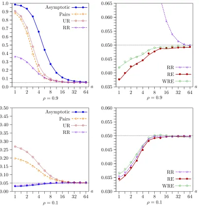
Figure1shows the effects of varyingafrom 1 (instruments very weak) to 64 (instruments extremely strong) by factors
Figure 1. Rejection frequencies as functions ofaforl−k=11 andn=400. Lines show results forts; symbols show results forth.
of√2. In these experiments,n=400 andl−k=11. The rea-sons for choosing these values will be discussed below. In the top two panels,ρ=0.9; in the bottom two,ρ=0.1. The left-hand panels show rejection frequencies for the asymptotic test and the pairs, UR, and RR bootstraps. The right-hand panels show rejection frequencies for the RE and WRE bootstraps, as well as partial ones for the RR bootstrap. Notice that the verti-cal axis is different in every panel and has a much larger range in the left-hand panels than in the right-hand ones. Results are shown for both the usualtstatistictsand the
heteroscedasticity-robust oneth. The former are shown as solid, dashed, or dotted
lines, and the latter are shown as symbols that are full or hollow circles, diamonds, or crosses.
Several striking results emerge from Figure1. In all cases, there is generally not much to choose between the results forts
and the results for th. This is not surprising, since the
dis-turbances are actually homoscedastic. Everything else we say about these results applies equally to both test statistics.
It is clear from the top left-hand panel that the older bootstrap methods (namely, the pairs, UR, and RR bootstraps) can overre-ject very severely whenρis large andais not large, although, in
this case, they do always work better than the asymptotic test. In contrast, the top right-hand panel shows that the new, effi-cient bootstrap methods (namely, the RE and WRE bootstraps) all tend to underreject slightly in the same case. This problem is more pronounced for RE than for WRE.
The two bottom panels show that, whenρis small, things can be very different. The asymptotic test now underrejects mod-estly for small values ofa, the pairs and UR bootstraps over-reject quite severely, and the RR bootstrap underover-rejects a bit less than the asymptotic test. This is a case in which bootstrap tests can evidently be much less reliable than asymptotic ones. As can be seen from the bottom right-hand panel, the efficient bootstrap methods generally perform much better than the older ones. There are only modest differences between the rejection frequencies for WRE and RE, with the former being slightly less prone to underreject for small values ofa.
It is evident from the bottom right-hand panel of Figure1 that the RR, RE, and WRE bootstraps perform almost the same whenρ=0.1, even when the instruments are weak. This makes sense, because there is little efficiency to be gained by run-ning regression (15) instead of regression (2) whenρ is small.
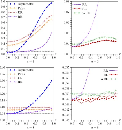
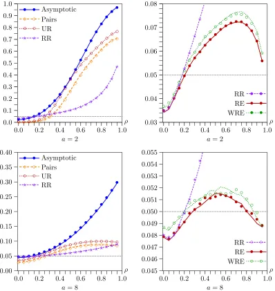
Figure 2. Rejection frequencies as functions ofρforl−k=11 andn=400. Lines show results forts; symbols show results forth.
Thus, we can expect the RE and RR bootstrap DGPs to be quite similar whenever the correlation between the reduced-form and structural disturbances is small.
Figure2 shows the effects of varyingρ from 0 to 0.95 by increments of 0.05. In the top two panels,a=2, so that the in-struments are quite weak, and, in the bottom two panels,a=8, so that they are moderately strong. As in Figure1, the two left-hand panels show rejection frequencies for older methods that often work poorly. We see that the asymptotic test tends to over-reject severely, except whenρ is close to 0, that the pairs and UR bootstraps always overreject, and that the RR bootstrap al-most always performs better than the pairs and UR bootstraps. However, even it overrejects severely whenρis large.
As in Figure1, the two right-hand panels in Figure2show re-sults for the new, efficient bootstrap methods, as well as partial ones for the RR bootstrap for purposes of comparison. Note the different vertical scales. The new methods all work reasonably well whena=2 and very well, although not quite perfectly, whena=8. Once again, it seems that WRE works a little bit better than RE.
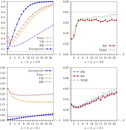
In the first two sets of experiments, the number of instru-ments is fairly large, with l−k=11, and different choices for this number would have produced different results. In Fig-ure3,l−kvaries from 1 to 21. In the top two panels, a=2 andρ =0.9; in the bottom two, a=2 andρ=0.1. Sincea is quite small, all the tests perform relatively poorly. As before, the new bootstrap tests generally perform very much better than the older ones, although, as expected, RR is almost indistin-guishable from RE whenρ=0.1.
Whenρ=0.9, the performance of the asymptotic test and the older bootstrap tests deteriorates dramatically as l−k in-creases. This is not evident whenρ=0.1, however. In contrast, the performance of the efficient bootstrap tests actually tends to improve asl−kincreases. The only disturbing result is in the top right-hand panel, where the RE and WRE bootstrap tests underreject fairly severely whenl=k≤3, that is, when there are two or fewer overidentifying restrictions. The rest of our experiments do not deal with this case, and so they may not ac-curately reflect what happens when the number of instruments is very small.
Figure 3. Rejection frequencies as functions ofl−kforn=400. Lines show results forts; symbols show results forth.
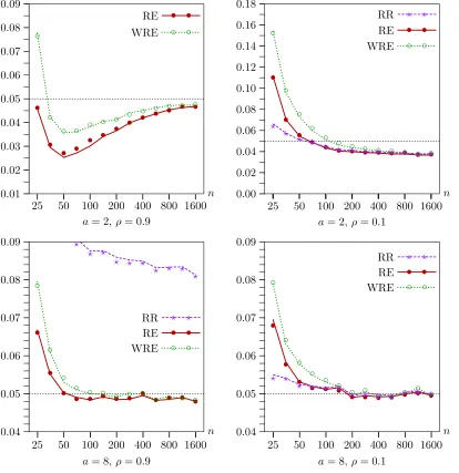
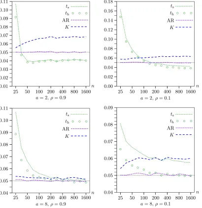
In all the experiments discussed so far, n=400. It makes sense to use a reasonably large number, because cross-section datasets with weak instruments are often fairly large. However, using a very large number would have greatly raised the cost of the experiments. Using larger values ofnwhile holdingafixed would not necessarily cause any of the tests to perform better, because, in theory, rejection frequencies approach nominal lev-els only as bothnandatend to infinity. Nevertheless, it is of interest to see what happens asnchanges while we holdafixed. Figure4shows how the efficient bootstrap methods perform in four cases (a=2 or a=8, and ρ=0.1 or ρ =0.9) for sample sizes that increase from 25 to 1600 by factors of ap-proximately√2. Note that, asnincreases, the instruments be-come very weak indeed whena=2. Forn=1600, theR2of the reduced-form regression (28) in the DGP, evaluated at the true parameter values, is just 0.0025. Even whena=8, it is just 0.0385.
The results in Figure4 are striking. Both the efficient boot-strap methods perform better forn=1600 than forn=25, of-ten very much better. Asnincreases from 25 to about 200, the
performance of the tests often changes quite noticeably. How-ever, their performance never changes very much asn is in-creased beyond 400, which is why we used that sample size in most of the experiments. When possible, the figure includes rejection frequencies for RR. Interestingly, whenρ=0.1, it ac-tually outperforms RE for very small sample sizes, although its performance is almost indistinguishable from that of RE for n≥70.
The overall pattern of the results in Figure4is in accord with the asymptotic theory laid out in Section3. In particular, the failure of the rejection frequency of the bootstrap t tests us-ing RE and WRE to converge to the nominal level of 0.05 as ngrows is predicted by that theory. The reason is that, under weak-instrument asymptotics, no estimate of a is consistent. Nevertheless, we see from Figure4that this inconsistency leads to an ERP of the bootstrap test fora=2 and largenthat is quite small. It is less than 0.004 in absolute value whenρ=0.9 and about 0.012 whenρ=0.1.
Up to this point, we have reported results only for equal-tail bootstrap tests, that is, ones based on the equal-tailp-value (8).
Figure 4. Rejection frequencies as functions ofnfork−l=11. Lines show results forts; symbols show results forth.
We believe that these are more attractive in the context oft sta-tistics than tests based on the symmetricp-value (7), because IV estimates can be severely biased when the instruments are weak. However, it is important to point out that results for sym-metric bootstrap tests would have differed, in some ways sub-stantially, from the ones reported for equal-tail tests.
Figure5 is comparable to Figure 2. It too shows rejection frequencies as functions ofρforn=400 andl−k=11, with a=2 in the top row anda=8 in the bottom row, but this time for symmetric bootstrap tests. Comparing the top left-hand pan-els of Figure5and Figure2, we see that, instead of overreject-ing, symmetric bootstrap tests based on the pairs and UR boot-straps underreject severely when the instruments are weak and
ρ is small, although they overreject even more severely than equal-tail tests whenρ is very large. Results for the RR boot-strap are much less different, but the symmetric version under-rejects a little bit more than the equal-tail version for small val-ues ofρand overrejects somewhat more for large values.
As one would expect, the differences between symmetric and equal-tail tests based on the new, efficient bootstrap methods
are much less dramatic than the differences for the pairs and UR bootstraps. At first glance, this statement may appear to be false, because the two right-hand panels in Figure 5 look quite different from the corresponding ones in Figure2. How-ever, it is important to bear in mind that the vertical axes in the right-hand panels are highly magnified. The actual differences in rejection frequencies are fairly modest. Overall, the equal-tail tests seem to perform better than the symmetric ones, and they are less sensitive to the values ofρ, which further justifies our choice to focus on them.
Next, we turn our attention to heteroscedasticity. The major advantage of the WRE over the RE bootstrap is that the former accounts for heteroscedasticity in the bootstrap DGP and the latter does not. Thus, it is of considerable interest to see how the various tests (now including AR andK) perform when there is heteroscedasticity.
In principle, heteroscedasticity can manifest itself in a num-ber of ways. However, because there is only one exogenous variable that actually matters in the DGP given by (27) and (28), there are not many obvious ways to model it without using a
Figure 5. Rejection frequencies as functions ofρfor symmetric bootstrap tests forl−k=11 andn=400. Lines show results forts; symbols show results forth.
more complicated model. In our first set of experiments, we used the DGP
y1=n1/2|w1| ∗u1, (29)
y2=aw1+u2, u2=ρn1/2|w1| ∗u1+rv, (30)
where, as before, the elements ofu1andvare independent and
standard normal. The purpose of the factor n1/2 is to rescale the instrument so that its squared length isninstead of 1. Thus, each element ofu1 is multiplied by the absolute value of the
corresponding element ofw1, appropriately rescaled.
We investigated rejection frequencies as a function ofρfor this DGP for two values ofa, namely, a=2 anda=8. Re-sults for the new, efficient bootstrap methods only are reported in Figure6. These results are comparable to those in Figure2. There are four test statistics (ts,th, AR, andK) and two
boot-strap methods (RE and WRE). The left-hand panels contain re-sults for a=2, and the right-hand panels for a=8. The top two panels show results for three tests that work badly, and the
bottom two panels show results for five tests that work at least reasonably well.
The most striking result in Figure6is that using RE, the boot-strap method which does not allow for heteroscedasticity, along with any of the test statistics that require homoscedasticity (ts,
AR, andK) often leads to severe overrejection. Of course, this is hardly a surprise. But the result is a bit more interesting if we express it in another way. UsingeitherWRE, the bootstrap method which allows for heteroscedasticity,orthe test statis-ticth, which is valid in the presence of heteroscedasticity of
un-known form, generally seems to produce rejection frequencies that are reasonably close to nominal levels.
This finding can be explained by the standard result, dis-cussed in Section3, under which bootstrap tests are asymptoti-cally valid whenever one of two conditions is satisfied. The first is that the quantity is asymptotically pivotal, and the second is that the bootstrap DGP converges in an appropriate sense to the true DGP. The first condition is satisfied by th but not by ts.
The second condition is satisfied by WRE but not by RE except when the true DGP is homoscedastic.
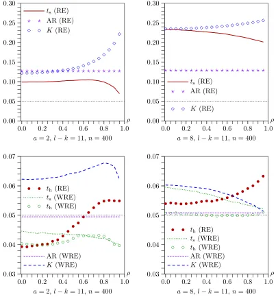
Figure 6. Rejection frequencies for four tests as functions ofρforl−k=11 andn=400 when disturbances are heteroskedastic.
Interestingly, the combination of the AR statistic and the WRE bootstrap works extremely well. Notice that rejection fre-quencies for AR do not depend onρ, because this statistic is solely a function ofy1. Whena=8, combining WRE withth
also performs exceedingly well, but this is not true whena=2. We also performed a second set of experiments in which the DGP was similar to (29) and (30), except that each element ofu1was multiplied byn1/2w21iinstead of byn1/2|w1i|. Thus, the heteroscedasticity was considerably more extreme. Results are not shown, because they are qualitatively similar to those in Figure6, with WRE continuing to perform well and RE per-forming very poorly (worse than in Figure6) when applied to the statistics other thanth.
The most interesting theoretical results of Section3deal with the asymptotic validity of the WRE bootstrap applied to AR, K,ts, andthunder weak instruments and heteroscedasticity. To
see whether these results provide a good guide in finite samples, we performed another set of experiments in which we varied the sample size from 25 to 1600 by factors of approximately√2
and used data generated by (29) and (30). Results for the usual four cases (a=2 ora=8 andρ=0.1 orρ=0.9) are shown in Figure7. Since the AR andKtests are not directional, upper-tail bootstrapp-values based on (7) were computed for them, while equal-tail bootstrapp-values based on (8) were computed for the twottests.
Figure7provides striking confirmation of the theory of Sec-tion3. The AR test not only demonstrates its asymptotic valid-ity but also performs extremely well for all sample sizes. As it did in Figure4,th performs well for large sample sizes when
a=8, but it underrejects modestly whena=2. The other tests are somewhat less satisfactory. In particular, theKtest performs surprising poorly in two of the four cases.
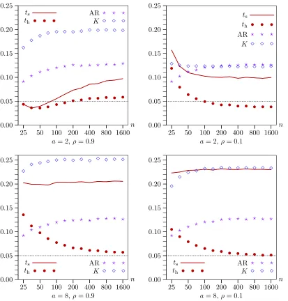
Figure8 contains results for the RE bootstrap for the same experiments as Figure 7. All of the tests exceptth now
over-reject quite severely for all sample sizes. Thus, as the theory predicts, only th is seen to be asymptotically valid for large
enough a. Careful examination of Figures 7 and8, which is a bit difficult because of the differences in the vertical scales,
Figure 7. Rejection frequencies for WRE bootstrap tests as functions ofnfork−l=11 when disturbances are heteroskedastic.
also shows that, for samples of modest size, thperforms
con-siderably better when bootstrapped using WRE rather than RE. This makes sense, since with WRE there is the possibility of an asymptotic refinement.
Taken together, our results for both the homoscedastic and heteroscedastic cases suggest that the safest approach is un-doubtedly to use the WRE bootstrap with the AR statistic. It is also reasonably safe to use the WRE bootstrap with the ro-busttstatisticthwhen the sample size is moderate to large (say,
200 or more) and the instruments are not extremely weak. Us-ing the RE bootstrap, or simply performUs-ing an asymptotic test, with any statistic except th can be very seriously misleading
when heteroscedasticity is present.
5. MORE THAN TWO ENDOGENOUS VARIABLES
Up to this point, as in Davidson and MacKinnon (2008), we have focused on the case in which there is just one endogenous variable on the right-hand side. The AR test (23), the K test, and the CLR test are designed to handle only this special case.
However, there is no such restriction for t statistics, and the RE and WRE bootstraps can easily be extended to handle more general situations.
For notational simplicity, we deal with the case in which there are just two endogenous variables on the right-hand side. It is trivial to extend the analysis to handle any number of them. The model of interest is
y1=β2y2+β3y3+Zγ+u1, (31) y2=Wπ2+u2, (32) y3=Wπ3+u3, (33)
where the notation should be obvious. As before,ZandWare, respectively, ann×kand ann×lmatrix of exogenous variables with the property thatS(Z)lies inS(W). For identification, we
require thatl≥k+2.
The pairs and UR bootstraps require no discussion. The RR bootstrap is also quite easy to implement in this case. To test the hypothesis that, say,β2=β20, we need to estimate by 2SLS
Figure 8. Rejection frequencies for RE bootstrap tests as functions ofnfork−l=11 when disturbances are heteroskedastic.
a restricted version of Equation (31),
y1−β20y2=β3y3+Zγ+u1, (34)
in whichy3is the only endogenous right-hand side variable, so
as to yield restricted estimatesβ3˜ andγ˜ and 2SLS residualsu˜1.
We also estimate Equations (32) and (33) by OLS, as usual. Then the bootstrap DGP is
y∗i1−β20y∗i2= ˜β3y∗3i+Ziγ˜+ ˜u∗1i,
y∗2i=Wiπˆ2+ ˆu∗2i, (35) y∗3i=Wiπˆ3+ ˆu∗3i,
where the bootstrap disturbances are generated as follows:
⎡ ⎣
˜ u∗1i ˆ u∗2i ˆ u∗3i
⎤ ⎦∼EDF
⎛ ⎝
˜ u1i
(n/(n−l))1/2uˆ2i
(n/(n−l))1/2uˆ3i
⎞
⎠. (36)
As before, we may omit the termZiγ˜ from the first of Equa-tions (35). In (36), we rescale the OLS residuals from the two
reduced-form equations but not the 2SLS ones from Equa-tion (34), although this is not essential.
For the RE and WRE bootstraps, we need to re-estimate Equations (32) and (33) so as to obtain more efficient estimates that are asymptotically equivalent to 3SLS. We do so by esti-mating the analogs of regression (15) for these two equations, which are
y2=Wπ2+δ2u˜1+residuals, and y3=Wπ3+δ3u˜1+residuals.
We then use the OLS estimates π˜2 andπ˜3 and the residuals
˜
u2≡y2−Wπ˜2andu˜3≡y3−Wπ˜3in the RE and WRE
boot-strap DGPs:
y∗i1−β20y∗i2= ˜β3y∗3i+Ziγ˜+ ˜u∗1i,
y∗2i=Wiπ˜2+ ˜u∗2i, (37) y∗3i=Wiπ˜3+ ˜u∗3i.
Only the second and third equations of (37) differ from the cor-responding equations of (35) for the RR bootstrap. In the case of the RE bootstrap, we resample from triples of (rescaled) resid-uals:
In the case of the WRE bootstrap, we use the analog of (19), which is
wherev∗i is a suitable random variable with mean 0 and vari-ance 1.
6. BOOTSTRAP CONFIDENCE INTERVALS
Every confidence interval for a parameter is constructed, im-plicitly or exim-plicitly, by inverting a test. We may always test whether any given parameter value is the true value. The upper and lower limits of the confidence interval are those values for which the test statistic equals its critical value. Equivalently, for an interval with nominal coverage 1−αbased on a two-tailed test, they are the parameter values for which thep-value of the test equalsα. For an elementary exposition, see Davidson and MacKinnon (2004, chap. 5).
There are many types of bootstrap confidence interval; Davi-son and Hinkley (1997) provided a good introduction. The type that is widely regarded as most suitable is the percentile t, or bootstrap t, interval. Percentiletintervals could easily be con-structed using the pairs or UR bootstraps, for which the boot-strap DGP does not impose the null hypothesis, but they would certainly work badly whenever bootstrap tests based on these methods work badly—that is, wheneverρis not small andais not large; see Figures1,2,3, and5.
It is conceptually easy, although perhaps computationally demanding, to construct confidence intervals using bootstrap methods that do impose the null hypothesis. We now explain precisely how to construct such an interval with nominal cover-age 1−α. The method we propose can be used with any boot-strap DGP that imposes the null hypothesis, including the RE and WRE bootstraps. It can be expected to work well when-ever the rejection frequencies for tests at levelαbased on the relevant bootstrap method are in fact close toα.
1. Estimate the model (1) and (2) by 2SLS so as to obtain the IV estimateβˆand the heteroscedasticity-robust standard error sh(β)ˆ defined in (6). Our simulation results suggest that there is no significant cost to using the latter rather than the usual stan-dard error that is not robust to heteroscedasticity, even when the disturbances are homoscedastic, for the sample sizes typically encountered with cross-section data.
2. Write a routine that, for any value of β, say β0, calcu-lates a test statistic for the hypothesis that β =β0 and
boot-straps it under the null hypothesis. This routine must performB bootstrap replications using a random number generator that de-pends on a seedmto calculate a bootstrapp-value, sayp∗(β0).
Forth, this should be an equal-tail bootstrapp-value based on
Equation (8). For the AR orKstatistics, it should be an upper-tail one.
3. Choose a reasonably large value ofBsuch thatα(B+1)is an integer, and also choosem. The same values ofmandBmust be used each timep∗(β0)is calculated. This is very important,
since otherwise a given value ofβ0would yield different values
ofp∗(β0)each time it was evaluated.
4. For the lower limit of the confidence interval, find two val-ues ofβ, sayβl−andβl+, withβl−< βl+, such thatp∗(βl−) <
α and p∗(βl+) > α. Since both values will normally be less thanβˆ, one obvious way to do this is to start at the lower limit of an asymptotic confidence interval, sayβl∞, and see whether p∗(βl)is greater or less thanα. If it is less than α, thenβl∞
can serve as βl−; if it is greater, then βl∞ can serve as βl+. Whichever ofβl−andβl+has not been found in this way can then be obtained by moving a moderate distance, perhapssh(β)ˆ ,
in the appropriate direction as many times as necessary, each time checking whether the bootstrapp-value is on the desired side ofα.
5. Similarly, find two values ofβ, say βu− and βu+, with
βu−< βu+, such thatp∗(βu−) > αandp∗(βu+) < α.
6. Find the lower limit of the confidence interval,βl∗. This is a value betweenβl−andβl+which is such thatp∗(βl∗)∼=α.
One way to findβl∗ is to minimize the function(p∗(β)−α)2
with respect toβin the interval[βl−, βl+]by using golden sec-tion search; see, for instance, Press et al. (2007, sec. 10.2). This method is attractive because it is guaranteed to converge to a local minimum and does not require derivatives.
7. In the same way, find the upper limit of the confidence interval,βu∗. This is a value betweenβu−andβu+which is such thatp∗(βu∗)∼=α.
When a confidence interval is constructed in this way, the limits of the interval have the property thatp∗(βl∗)=∼p∗(βu∗)∼= α. The approximate equalities here would become exact, sub-ject to the termination criterion for the golden search routine, ifBwere allowed to tend to infinity. The problem is thatp∗(β)
is a step function, the value of which changes by precisely 1/B at certain points as its argument varies. This suggests thatB should be fairly large, if possible. It also rules out the many numerical techniques that, unlike golden section search, use in-formation on derivatives.
7. AN EMPIRICAL EXAMPLE
The method of instrumental variables is routinely used to an-swer empirical questions in labor economics. In such applica-tions, it is common to employ fairly large cross-section datasets for which the instruments are very weak. In this section, we ap-ply our methods to an empirical example of this type. It uses the same data as Card (1995). The dependent variable in the structural equation is the log of wages for young men in 1976, and the other endogenous variable is years of schooling. There are 3,010 observations without missing data, which originally came from the Young Men Cohort of the National Longitudinal Survey.
Although we use Card’s data, the equation we estimate is not identical to any of the ones he estimates. We simplify the speci-fication by omitting a large number of exogenous variables hav-ing to do with location and family characteristics, which appear to be collectively insignificant, at least in the IV regression. We
also use age and age squared instead of experience and experi-ence squared in the wage equation. As Card noted, experiexperi-ence is endogenous if schooling is endogenous. In some specifica-tions, he therefore used age and age squared as instruments. For purposes of illustrating the methods discussed in this arti-cle, it is preferable to have just two endogenous variables in the model, and so we do not use experience as an endogenous re-gressor. This slightly improves the fit of the IV regression, but it also has some effect on the coefficient of interest. In addition to age and age squared, the structural equation includes a constant term and dummies for race, living in a southern state, and living in an SMSA as exogenous variables.
We use four instruments, all of which are dummy variables. The first is 1 if there is a two-year college in the local labor market, the second if there is either a two-year college or a four-year college, the third if there is a public four-four-year college, and the fourth if there is a private four-year college. The second instrument was not used by Card, although it is computed as the product of two instruments that he did use. The instruments are fairly weak, but apparently not as weak as in many of our simulations. The concentration parameter is estimated to be just 19.92, which is equivalent toa=4.46. Of course, this is just an estimate, and a fairly noisy one. The Sargan statistic for overi-dentication is 7.352. This has an asymptoticp-value of 0.0615 and a bootstrapp-value, using the wild bootstrap for the unre-stricted model, of 0.0658. Thus, there is weak evidence against the overidentifying restrictions.
Our estimate of the coefficientβ, which is the effect of an additional year of schooling on the log wage, is 0.1150. This is higher than some of the results reported by Card and lower than others. The standard error is either 0.0384 (assuming ho-moscedasticity) or 0.0389 (robust to heteroscedasticity). Thus the t statistics for the coefficientβ to be zero and the corre-sponding asymptoticp-values are:
ts=2.999 (p=0.0027) and
th=2.958 (p=0.0031).
Equal-tail bootstrapp-values are very similar to the asymptotic ones. Based onB=99,999, the p-value is 0.0021 for the RE bootstrap usingts, and either 0.0021 or 0.0022 for the WRE
bootstrap usingth. The first of these wild bootstrapp-values is
based on the Rademacher distribution (21) that imposes sym-metry, and the second is based on the distribution (20) that does not.
We also compute the AR statistic, which is 5.020 and has a p-value of 0.00050 based on the F(4,3,000) distribution. WRE bootstrapp-values are 0.00045 and 0.00049 based on (21) and (20), respectively. It is of interest that the AR statistic re-jects the null hypothesis even more convincingly than the boot-straptstatistics. As some of the simulation results in Davidson and MacKinnon (2008) illustrate, this can easily happen when the instruments are weak. In contrast, thep-values for the K statistic, which is 7.573, are somewhat larger than the ones for thetstatistics. The asymptoticp-value is 0.0059, and the WRE ones are 0.0056 and 0.0060.
Up to this point, our bootstrap results merely confirm the as-ymptotic ones, which suggest that the coefficient of schooling is almost certainly positive. Thus, they might incorrectly be taken
to show that asymptotic inference is reliable in this case. In fact, it is not. Since there is a fairly low value ofaand a reasonably large value ofρ(the correlation between the residuals from the structural and reduced-form equations is−0.474), our simula-tion results suggest that asymptotic theory should not perform very well in this case. Indeed, it does not, as becomes clear when we examine bootstrap confidence intervals.
We construct 11 different 0.95 confidence intervals for β. Two are asymptotic intervals based ontsandth, two are
asymp-totic intervals obtained by inverting the AR and K statistics, and seven are bootstrap intervals. The procedure for inverting the AR andK statistics is essentially the same as the one dis-cussed in Section6, except that we use either theF(4,3,000)or
χ2(1)distributions instead of a bootstrap distribution to com-putep-values. One bootstrap interval is based ontswith the RE
bootstrap. The others are based onth, AR, andK, each with two
different variants of the WRE bootstrap. The “s” variant uses (21) and thus imposes symmetry, while the “ns” variant uses (20) and thus does not impose symmetry. In order to minimize the impact of the specific random numbers that were used, all bootstrap intervals are based onB=99,999. Each of them re-quired the calculation of at least 46 bootstrapp-values, mostly during the golden section search. Computing each bootstrap in-terval took about 30 minutes on a Linux machine with an Intel Core 2 Duo E6600 processor.
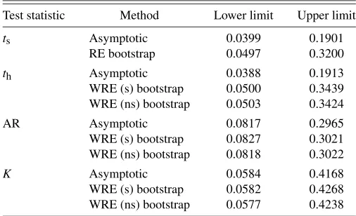
It can be seen from Table1that, for thetstatistics, the lower limits of the bootstrap intervals are moderately higher than the lower limits of the asymptotic intervals, and the upper limits are very much higher. What seems to be happening is thatβˆis biased downwards, becauseρ <0, and the standard errors are also too small. These two effects almost offset each other when we test the hypothesis thatβ=0, which is why the asymptotic and bootstrap tests yield such similar results. However, they do not fully offset each other for the tests that determine the lower limit of the confidence interval, and they reinforce each other for the tests that determine the upper limit.
All the confidence intervals based on the AR statistic are sub-stantially narrower than the bootstrap intervals based on the t statistics, although still wider than the asymptotic intervals based on the latter. In contrast, the intervals based on the K statistic are even wider than the bootstrap intervals based on thetstatistics. This is what one would expect based on thep -values for the tests ofβ=0. Of course, if the overidentifying
Table 1. Confidence intervals forβ
Test statistic Method Lower limit Upper limit
ts Asymptotic 0.0399 0.1901 RE bootstrap 0.0497 0.3200
th Asymptotic 0.0388 0.1913 WRE (s) bootstrap 0.0500 0.3439 WRE (ns) bootstrap 0.0503 0.3424 AR Asymptotic 0.0817 0.2965 WRE (s) bootstrap 0.0827 0.3021 WRE (ns) bootstrap 0.0818 0.3022
K Asymptotic 0.0584 0.4168 WRE (s) bootstrap 0.0582 0.4268 WRE (ns) bootstrap 0.0577 0.4238