Full Terms & Conditions of access and use can be found at
http://www.tandfonline.com/action/journalInformation?journalCode=ubes20
Download by: [Universitas Maritim Raja Ali Haji] Date: 12 January 2016, At: 01:06
Journal of Business & Economic Statistics
ISSN: 0735-0015 (Print) 1537-2707 (Online) Journal homepage: http://www.tandfonline.com/loi/ubes20
Comparing the Point Predictions and Subjective
Probability Distributions of Professional
Forecasters
Joseph Engelberg, Charles F. Manski & Jared Williams
To cite this article: Joseph Engelberg, Charles F. Manski & Jared Williams (2009) Comparing the Point Predictions and Subjective Probability Distributions of Professional Forecasters, Journal of Business & Economic Statistics, 27:1, 30-41, DOI: 10.1198/jbes.2009.0003
To link to this article: http://dx.doi.org/10.1198/jbes.2009.0003
Published online: 01 Jan 2012.
Submit your article to this journal
Article views: 329
View related articles
Comparing the Point Predictions and
Subjective Probability Distributions of
Professional Forecasters
Joseph E
NGELBERGKenan-Flagler Business School, University of North Carolina, Chapel Hill, NC 27599 (joseph_engelberg@kenan-flagler. unc.edu)
Charles F. M
ANSKIDepartment of Economics and Institute for Policy Research, Northwestern University, Evanston, IL 60208 (cfmanski@northwestern.edu)
Jared W
ILLIAMSSmeal College of Business, Pennsylvania State University, University Park, PA 16802 (jmw52@psu.edu)
We use data from the Survey of Professional Forecasters (SPF) to compare point predictions of gross domestic product (GDP) growth and inflation with the subjective probability distributions held by fore-casters. We find that most SPF point predictions are quite close to the central tendencies of forecasters’ subjective distributions. We also find that the deviations between point predictions and the central tendencies of forecasters’ subjective distributions tend to be asymmetric, with SPF forecasters tending to report point predictions that give a more favorable view of the economy than do their subjective means/medians/modes. KEY WORDS: Point estimates; Probabilistic questions; Professional forecasters; Subjective probability
distributions; Survey methods; Survey of professional forecasters.
1. INTRODUCTION
Professional forecasters have long given point predictions of future events. Financial analysts offer point predictions of the profit that firms will earn in the quarter ahead, macroeconomic forecasters give point predictions of annual gross domestic product (GDP) growth and inflation, and film critics conjecture which actors will win Academy Awards. A notable exception is that meteorologists commonly report the chance that it will rain during the next day. However, meteorologists give point rather than probabilistic predictions of the next day’s high and low temperatures.
Thoughtful forecasters rarely think that they have perfect foresight. Hence, their point predictions can at most convey some notion of the central tendency of their beliefs, and nothing at all about the uncertainty they feel. It has been standard in economics to assume that persons use subjective probability distributions to express uncertainty about future events. Suppose that forecasters actually have subjective probability distributions for the events they predict. Then their point predictions should somehow be related to their subjective distributions. But how? This is the question that we address.
When the forecasting problem is to predict the occurrence of a binary event, the idea that point predictions should somehow be related to subjective probability distributions was suggested 40 years ago by Juster (1966). Considering the case in which consumers are asked to give a point prediction of their buying intentions (buy or not buy), Juster wrote (page 664): ‘‘Con-sumers reporting that they ‘intend to buy Awithin X months’ can be thought of as saying that the probability of their purchasing A within X months is high enough so that some form of ‘yes’ answer is more accurate than a ‘no’ answer.’’ Thus, he
hypoth-esized that a consumer facing a yes/no intentions question responds as would a statistician asked to make a best point prediction of a future random event. Subsequent analysis for-malizing Juster’s idea appears in Manski (1990).
Our concern is prediction of real-valued outcomes such as firm profit, GDP growth, or temperature. In these cases, the users of point predictions sometimes presume that forecasters report the means of their subjective probability distributions, that is, their best point predictions under square loss. However, forecasters are not specifically asked to report subjective means. Nor are they asked to report subjective medians or modes, which are best predictors under other loss functions. Instead, they are simply asked to ‘‘predict’’ the outcome or to provide their ‘‘best prediction,’’ without definition of the word ‘‘best.’’ In the absence of explicit guidance, forecasters may report different distributional features as their point predictions. Some may report subjective means, others subjective medians or modes, and still others, applying asymmetric loss functions, may report various quantiles of their subjective probability distributions.
It is important to understand reporting practices, because they can be consequential for the interpretation of point pre-dictions. It is possible that forecasters who hold identical probabilistic beliefs provide different point predictions and forecasters with dissimilar beliefs provide identical point pre-dictions. If so, comparison of point predictions across fore-casters is problematic. Variation in predictions need not imply disagreement among forecasters, and homogeneity in pre-dictions need not imply agreement.
30
2009 American Statistical Association Journal of Business & Economic Statistics January 2009, Vol. 27, No. 1 DOI 10.1198/jbes.2009.0003
To perform our analysis requires a data source in which forecasters provide both point predictions and subjective dis-tributions for specific events. Almost uniquely among existing forecasting instruments, the Survey of Professional Forecasters (SPF) provides such data (www.phil.frb.org/econ/spf/). The SPF respondents are macroeconomic forecasters who are queried about future GDP growth and inflation in the United States. The forecasters provide both point and probabilistic predictions for these quantities; the latter are the probabilities that the outcome will lie in each of ten intervals. Another important feature of the SPF is that the survey has a longi-tudinal component, with many forecasters providing multiple predictions over the course of several years. Section 2 describes the SPF data in detail.
Although the SPF probabilistic forecasts do not completely identify the subjective distributions that respondents hold, they do imply fairly tight bounds on the means, medians, and modes of these distributions. Hence, we are able to compare re-spondents’ point predictions with these features of their sub-jective probability distributions. This is done in Section 3.
We report two primary findings. First, most SPF point pre-dictions are quite close to the central tendencies of forecasters’ subjective distributions. At least 1,343 out of 1,623 GDP growth predictions and 1,296 out of 1,550 inflation forecasts lie within 1% of forecasters’ subjective medians for these out-comes. Most point predictions are similarly close to fore-casters’ subjective means and modes, as these typically are close to the subjective medians. The closeness of the point predictions and the three measures of central tendency would be unremarkable if the subjective distributions were tightly concentrated. However, the probabilistic forecasts often exhibit considerable spread, with about 40% of the forecasts placing positive probability mass in four or more intervals. Thus, the SPF forecasters express clear uncertainty about future GDP growth and inflation.
Second, the deviations between point predictions and the central tendencies of forecasters’ subjective distributions tend to be asymmetric. In particular, SPF forecasters tend to report point predictions that give a more favorable view of the economy than do their subjective means/medians/modes. In the case of GDP growth, respondents who give point predictions outside the bounds that we obtain for their subjective means/ medians/modes are more likely to report point predictions that are above the upper bound than below the lower bound. In the case of inflation, the point predictions are more often below the lower bounds than above the upper bounds. We also find per-sistence over time in the reporting practices of individual respondents: forecasters who give point predictions above/ below their subjective means/medians/modes in one sample period are more likely to do the same the next period. In an Appendix, we perform a robustness check that reinforces these findings. For further analysis of the type we present here, see Clements (2007), who applies our bounding approach to study whether forecasters’ point expectations of a future decline in output are consistent with their subjective proba-bility distributions.
Both of the primary findings are apparent when we compare the standard SPF ‘‘consensus’’ projections for the economy with alternative consensus projections that we derive from the
probabilistic forecasts. The standard consensus projections are the median point predictions of respondents. The alternative consensus projections are approximately the cross-sectional medians of respondents’ subjective medians (see Section 3 for the exact definition). Considering the period 1992–2004, we find that the two versions of consensus projection have the same qualitative time series variation and, on average, are within .0025 of one another. However, to the extent that the two time series differ, the standard consensus projection tends to give a slightly more favorable view of the economy than does the alternative.
The analysis described previously is nonparametric—we use the SPF interval probability data in their raw form to bound subjective means/medians/modes rather than to fit the precise subjective probability distributions that respondents hold. In Section 4, we suppose that each subjective distribution placing positive probability on at least three intervals has the general-ized Beta form, and we use the interval probability data to fit the parameters. In those cases where a forecast places positive probability on only one or two intervals, we suppose that the distribution has the shape of an isosceles triangle and we fit its parameters. This done, we are able to compare SPF point predictions with the fitted probability distributions. The para-metric analysis corroborates and sharpens our nonparapara-metric comparison of point predictions and probabilistic forecasts.
Considering the logic of point prediction and probabilistic forecasting, we suggest that the SPF and similar surveys should emphasize probabilistic forecasts and, perhaps, should not bother asking for point predictions at all. As demonstrated here, it is easy enough to extract well-defined point predictions from the SPF probabilistic forecasts, for example, by taking the point prediction to be a respondent’s subjective median. In contrast, one can never be sure what feature of the subjective distribution an SPF forecaster has in mind when he reports a point pre-diction directly. In the finance literature, researchers have interpreted cross-forecaster dispersion in point predictions to indicate disagreement in their beliefs (e.g., Diether, Malloy, and Scherbina, 2002; Mankiw, Reis, and Wolfers, 2003). We caution that this research practice confounds variation in forecaster beliefs with variation in the manner that forecasters make point predictions.
Even if point predictions were fully successful in describing the central tendencies of SPF forecaster beliefs, they inherently would reveal nothing about the uncertainty that forecasters feel when predicting GDP growth or inflation. Probabilistic fore-casts are well-suited to this task. Although economists have long assumed that persons use subjective distributions to express uncertainty, an empirical literature eliciting subjective distributions has developed more recently. Since the early 1990s, economists engaged in survey research have increas-ingly asked respondents to report probabilistic expectations of future economic events, including stock market returns, job loss, earnings, and Social Security benefits. Manski (2004) reviews recent research eliciting probabilistic expectations in surveys and assesses the state of the art.
A separate matter, which we do not feel the need to address in the body of our article, is the longstanding use of cross-sectional dispersion in point predictions to measure forecaster uncertainty about future outcomes. See, for example, Cukierman
and Wachtel (1979), Levi and Makin (1979, 1980), Makin (1982), Brenner and Landskroner (1983), Hahm and Steigerwald (1999), and Hayford (2000). This research practice is suspect on logical grounds, even if all forecasters make their point predictions in the same way. Even in the best of cir-cumstances, point predictions provide no information about the uncertainty that forecasters feel. This point was made force-fully 20 years ago by Zarnowitz and Lambros (1987). Never-theless, some researchers have continued since then to use the dispersion in point predictions to measure forecaster uncertainty.
Even though Zarnowitz and Lambros (1987) explicitly rec-ognized the logical fallacy in using the dispersion in point predictions to measure forecaster uncertainty, they nevertheless thought it useful to determine the empirical relationship between such dispersion and uncertainty among the SPF respondents. More recently, Giordani and Soderlind (2003) have performed a similar empirical analysis. As far as we are aware, the Zarnowitz and Lambros (1987) and Giordani and Soderlind (2003) papers are the only research before our own that has compared the SPF point and probabilistic predictions. However, their analyses differ fundamentally from ours. They sought to describe the empirical relationship between the cross-sectional distribution of point predictions and the uncertainty evident in a typical forecaster’s subjective probability dis-tribution. In contrast, our concern is to understand the empirical relationship betweenindividual forecasters’ point predictions and their subjective probability distributions.
2. DATA
Our data are from the SPF, administered since 1990 by the Federal Reserve Bank of Philadelphia. The SPF was begun in 1968 by the American Statistical Association and the National Bureau of Economic Research; hence, it was originally called the ASA-NBER survey. The panel of forecasters, who include university professors and private-sector macroeconomic researchers, are asked to predict American GDP, inflation, unemployment, interest rates, and other macroeconomic vari-ables. The survey, which is performed quarterly, is mailed to panel members the day after the government release of quar-terly data on the national income and product accounts. The composition of the panel changes gradually over time, with individual members providing forecasts for about six years on average.
2.1 Question Format
Each quarter, the SPF asks panel members to make point and probabilistic forecasts of annual real GDP and inflation. To analyze the responses, it is important to understand the specific format of the questions. We explain the point and probabilistic questions in turn.
2.1.1 Point Predictions. The SPF instrument provides the value of GDP in the previous calendar year and asks for a point prediction of GDP in the current and the next year. Thus, in the four quarterly surveys administered during calendar year t, respondents are told the value of real GDP in yeart1 and are asked to give point predictions of annual GDP in years tand
tþ1. Similarly, the instrument provides the average value of the GDP price index in the previous calendar year and asks for a point prediction of the average GDP price index in the current and the next year. The instrument does not specify how respondents should form their point predictions. In particular, it does not ask for means, medians, or modes.
2.1.2 Probabilistic Forecasts. In the four quarterly sur-veys administered during calendar year t, respondents are asked to forecast the percentage change in annual real GDP between yearst1 andtand, likewise, the percentage change in GDP between yearstandtþ1. They are similarly asked to forecast year-to-year percentage changes in the average GDP price index. In each case, the SPF instrument partitions the real number line into intervals and asks respondents to report their subjective probabilities that the variable of interest will take a value in each interval. For GDP growth, the intervals are (‘,
2%), [x%,xþ1%) forx¼ 2,1,. . ., 5, and [6%,‘). For
inflation they are (‘, 0%), [x%,xþ1%) forx¼0, 1,. . ., 7
and [8%,‘).
Observe that panel members are asked to give point pre-dictions of the levels of GDP and the GDP price index, but probabilistic forecasts of the year-to-year percentage changes in these quantities. To make the point predictions comparable to the probabilistic ones, we must convert the point predictions of levels into point predictions of percentage change. This is straightforward to do between yearst 1 and t, because the SPF instrument tells respondents the actual value of the year
t1 level. Thus, to obtain a forecaster’s point prediction of the percentage change in GDP between yearst1 andt, we calculate the percentage change between the SPF-specified level of yeart1 GDP and the respondent’s point prediction of yeartGDP. This calculation is correct provided that panel members accept as accurate the SPF figure for yeart1 GDP. During yeartinformation about yeart1 GDP and the GDP price index continues to be collected by the government. Therefore, yeart1 values for GDP and the price index often are revised from quarter to quarter. The SPF updates the figures it gives forecasters accordingly. These revisions were generally small during our 1992–2004 sample period, the one notable exception being a large revision in both accounts due to an accounting overhaul of the National Income and Product Accounts in quarter 4 of 1999. Otherwise, the average absolute value of the revision from quarter 1 to quarter 2 was 0.05% for GDP and 0.03% for the price index, from quarter 2 to quarter 3 was 0.37% for GDP and 0.22% for the price index, and from quarter 3 to quarter 4 was 0.12% for GDP and .02% for the price index. There were only four cases for GDP and no cases for the price index where the change between quarters was larger than 1%. It is not straightforward to produce point predictions of percentage change between yearstandtþ1. In this case, we only know forecasters’ point predictions of the levels for the two years, and these point predictions are related in unknown ways to their subjective distributions. Hence, the percentage change in point predictions between yearstandtþ1 need not equal the point prediction for percentage change that a panel member would have stated had he been asked this question.
To see this consider a forecaster who (1) believes that annual inflation will be 10% with probability 0.4 and 0% with prob-ability 0.6, (2) believes that annual inflation rates are serially
independent, and (3) uses the absolute loss function (so his point prediction is the median of his subjective probability distribution). Suppose the price index level at yeart1 is 1. Then the forecaster will provide the estimates 1 and 1.1 for the price index levels for yearstandtþ1, respectively, because these are the medians of his subjective probability distributions for inflation rates in years t and t þ 1. Notice that the per-centage change in the forecaster’s point predictions for the price index level between years t and year t þ 1 is
ð1:11Þ=1¼10%, but if the forecaster were asked for his point prediction for the inflation rate in yeartþ1, he would say ‘‘0%.’’ The same problem arises when one tries to compare quarterly point predictions with annual probabilistic forecasts. Because of this, we do not try to match forecasters’ point predictions for year t þ 1 index levels with their subjective probability distributions for GDP growth and inflation; rather, we restrict attention to yeartpoint predictions and subjective probability distributions.
2.2 Sample for Analysis
Although the SPF began in 1968, we restrict attention to data collected from 1992 on. There are several reasons for this:
1. The survey only began asking forecasters for their annual (rather than quarterly) point predictions in the third quarter of 1981. This is important since the probabilistic forecasts are for annual changes.
2. After the third quarter of 1981, the survey intended to ask forecasters to report point predictions for current and next year’s GDP. However, the Philadelphia Fed has identified a few surveys between 1985 and 1990 in which it appears that forecasters were mistakenly asked about the previous and current year GDP instead. The Fed took over the survey in Quarter 2 of 1990 and is sure that none of the surveys since then have these errors. 3. The intervals in which respondents place probabilities have changed over the years. From Quarter 3 of 1981 through the end of 1991, there were 6 intervals, and after 1991, there were 10 intervals.
4. The administrators of the SPF do not know whether respondents were provided figures for the previous year’s GDP
and GDP price index prior to Quarter 3 of 1990. Our method of converting point predictions of levels into point predictions of percentage changes is only valid if respondents are given this information.
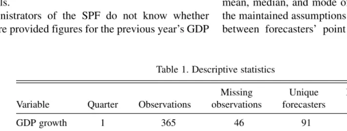
We restrict our analysis to the survey responses between Quarter 1 of 1992 and Quarter 4 of 2004. We also exclude Quarter 1 of 1996 since the previous-year values were unknown at the time because of a delay in the release of the data caused by the federal government shutdown. As Table 1 demonstrates, even after this restriction our sample is large, with 3,173 observations provided by 116 unique forecasters over the 13-year period.
In contrast with other papers that use the entire available SPF time series, our restriction to the post-1991 surveys and the yeart1 andtforecasts represents a conscious effort to use the cleanest possible data and methodology. The data we use enable us to avoid (1) using functions of quarterly point pre-dictions to construct an annual point prediction and (2) using functions oftandtþ1 point predictions to construct a point prediction of percentage change from t tot þ1. These con-structions are valid only if forecasters’ point predictions relate to their subjective distributions in certain ways, in particular, if they are subjective means. Given that the purpose of this paper is to explore the relationship between point predictions and probabilistic forecasts, it seems unwise to assume any rela-tionship a priori. Moreover, the post-1991 data avoid the survey errors in the pre-1992 period and the larger bins in the 1981– 1991 periods, which provide far less information about fore-casters’ subjective distributions.
3. NONPARAMETRIC ANALYSIS
Our analysis maintains the standard economic assumption that forecasters use subjective probability distributions to express their uncertainty about future events. We assume that the probabilistic forecasts reported in the SPF accurately describe these subjective distributions. In probability theory, the three most prominent measures of central tendency are the mean, median, and mode of a distribution. The SPF data and the maintained assumptions enable us to study the relationship between forecasters’ point predictions and these measures.
Table 1. Descriptive statistics
GDP growth 2 430 49 105 33.1
GDP growth 3 414 47 103 31.8
GDP growth 4 414 54 97 31.8
Inflation 1 347 64 88 28.9
Inflation 2 412 67 100 31.7
Inflation 3 395 66 99 30.4
Inflation 4 396 72 94 30.5
ALL — 3,173 465 116 31.1
NOTE: We count an observation as missing if (1) the forecaster does not provide a current year level point estimate or (2) the forecaster does not provide values for his subjective distribution. Of our 3,173 observations, 5 had probabilities that did not sum to 100%. They summed to 99.7%, 99.9%, 100.2%, 100.2%, and 100.4%. Because these differences were so small, we did not exclude any of these observations.
The analysis is in two parts. In this section, we perform a nonparametric analysis that does not assume subjective distributions to have any specific shape. In Section 4, we sup-pose that each subjective distribution has a Beta or isosceles-triangle shape, and we reconsider the data from that perspective. Before beginning we think it important to call attention to the fact that views have varied on the proper interpretation of expectations elicited in surveys, whether they be probabilistic forecasts, point predictions, or verbal statements of likelihood. As discussed in Manski (2004), the matter has long been a subject of controversy, both within and across the disciplines of cognitive psychology and economics. The controversy persists because one can never be sure that forecasts elicited in surveys reveal what people ‘‘really think.’’
An example arose in the review of this article, when an anonymous reviewer hypothesized that SPF forecasters might give more careful consideration to their point predictions than to their probabilistic forecasts. Of course, one might just as well pose the opposite hypothesis. The language that we use in reporting our analysis reflects our presumptions that (1) the SPF probabilistic and point predictions are both the result of careful deliberation and (2) heterogeneity across forecasters in the relationship between their probabilistic and point forecasts reflects heterogeneity in the loss functions that they apply to their subjective distributions.
A reader who wishes to remain agnostic can learn intriguing empirical facts from the analysis without necessarily having to accept our interpretation. There also is clear merit in per-forming robustness checks that weaken or modify the assumptions that we maintain. We present one such check in an Appendix. There we loosen the assumption that the proba-bilistic forecasts reported in the SPF describe forecasters’ subjective distributions with full accuracy and instead consider the possibility that respondents round their probabilistic fore-casts to multiples of .05. We then perform again key parts of the analysis of Section 3 and report the findings.
3.1 Bounding Means, Medians, and Modes
Recall that the SPF probabilistic questions ask forecasters to report their subjective probabilities that GDP growth and inflation will lie in given intervals on the real line. The responses to these questions do not fully reveal the subjective distributions that respondents hold, but they do bound these distributions. The data directly imply bounds on subjective means and medians. These bounds are most easily explained by way of examples.
Consider the SPF questions concerning inflation. Respond-ents are asked for 10 subjective probabilities: the probability that prices will decline; the probabilities that the percentage inflation rate, denotedi, will lie in the interval [x,xþ1) forx¼
0, 1,. . ., 7%; and the probability that the inflation rate will be 8% or higher. Suppose that a forecaster gives these positive responses:P(0#i< 1)¼0.2,P(1#i< 2)¼0.2,P(2#i< 3)¼
0.3,P(3#i< 4)¼0.2, andP(4#i< 5)¼0.1, with all other responses being zero. Then we can immediately conclude that this forecaster’s subjective median for inflation lies in the interval [0.02, 0.03). Lower and upper bounds on this sub-jective mean are obtained by placing all of each interval’s
probability mass at the interval’s lower and upper endpoint, respectively. The resulting bound is [0.018, 0.028).
These bounds on the median and mean are finite intervals of width 0.01, but there are other examples in which the bounds are infinite. Consider a forecaster with strong bimodal expectations who states thatP(i< 0)¼0.4 andP(8#i)¼0.6. In this case, we can only conclude that the subjective median is larger than 0.08 and we cannot conclude anything at all about the subjective mean. Fortunately, for our analysis, cases with bounds of infinite width occur only occasionally. Of the 3,173 probabilistic forecasts that we observe, none yield a bound of infinite width on the forecaster’s subjective median, and 363 yield a bound of infinite width on the subjective mean. In all other cases, the bound on the median and mean has width 0.01. Using the SPF data to bound the mode of a subjective dis-tribution is more subtle, because the mode is a local property that cannot be inferred from interval data without imposing some assumption. Our analysis assumes that the mode is contained in the interval with the greatest probability mass. Thus, we conclude in the preceding first example that the mode lies in the interval [0.02, 0.03) and in the second that it lies in the interval [0.08,‘). In some cases, multiple intervals have the
same greatest probability mass; for example, this would have occurred in the first example if the forecaster had placed probability 0.3 on both of the intervals [0.02, 0.03) and [0.03, 0.04). Of the 3,173 forecasts, none yield a bound of infinite width on the forecaster’s subjective mode and 243 yield a finite bound of width greater than 0.01. In all other cases, the bound on the mode has width 0.01.
Although the bounds cannot pinpoint the mean/median/mode of each subjective distribution, they typically have width 0.01 and, hence, are very informative. Examination of the bounds shows that, in most cases, the three measures of central tendency are fairly close to one another. Calculations not reported here show that, in three quarters of the cases, the distance separating the three measures must be no larger than 0.015.
3.2 Consistency of Point Predictions with the Bounds
Having computed the preceding bounds, now consider a forecaster’s point prediction of some quantity. If the point prediction lies within the bound for the median, then we cannot reject the hypothesis that the point prediction is the median. If the point prediction does not lie within the bound for the median, we can reject this hypothesis. The same reasoning applies to the mean and mode. Thus, we can determine the frequency with which point predictions are and are not con-sistent with the three measures of central tendency.
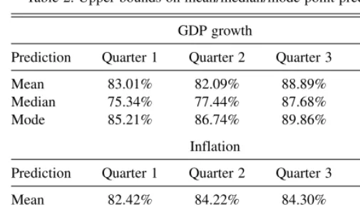
Table 2 gives the findings, aggregated across the years 1992– 2004 but disaggregated by quarter. Each entry in the table gives the percentage of cases in which a panel member’s point pre-diction of a given quantity in a given quarter lies within his bound for a given measure of central tendency. For example, the upper left entry for GDP growth, which is 83.01%, means that 83.01% of all first-quarter GDP point predictions lay within the bound obtained for the forecaster’s subjective mean. We call this an ‘‘Upper Bound on Mean Point Prediction,’’ be-cause consistency of a point prediction with a bound does not imply that the forecaster must have given his subjective mean as
his point prediction. It only implies that he may have given the subjective mean.
The table shows that most point predictions are consistent with the hypotheses that SPF panel members report their sub-jective means, medians, or modes. However, there are many panel members whose point predictions are inconsistent with these hypotheses. This is especially evident in Quarter 1, where (17%, 25%, 15%) percent of the respondents give point pre-dictions that cannot be their subjective mean/median/mode.
Observe that, in each row of the table, the entries in the table increase markedly from Quarter 1 to Quarter 4. This is rea-sonable to expect, because the forecast horizon shrinks as the year goes on—while most of the current year lies ahead in the Quarter 1 surveys, most of it lies behind when the Quarter 4 surveys are conducted. Thus, the SPF forecasters should tend to have sharper subjective distributions in Quarter 4 than in Quarter 1, implying that alternative measures of central ten-dency should draw nearer to one another.
Table 3 shows that subjective distributions do tend to sharpen as the year goes on. For each quarter and quantity of interest, the table shows the percentage of forecasters whose positive probability assessments are concentrated inNor fewer intervals, whereNranges from 1 to 10. Observe how the entries increase with Quarter. Consider, for example, the column forN
¼2 when the quantity is GDP growth. In Quarter 1, only 6.9%
of the forecasters have subjective distributions that are con-centrated in two or fewer intervals. In Quarter 4, beliefs have sharpened so much that 58.9% of the subjective distributions are this concentrated.
3.3 Inconsistencies Tend to Present Favorable Scenarios
Now consider the SPF panel members whose point pre-dictions are not consistent with their subjective means, medians, or modes. Table 4 reports the percentage of such cases in which the point prediction lies below or above the bound. A clear finding emerges. Most such point predictions give a view of the economy that is favorable relative to the central tendencies of respondents’ subjective distributions. Thus, forecasters who skew their point predictions tend to present rosy scenarios.
The table shows that, when forecasting GDP, the point pre-dictions that are inconsistent with measures of central tendency are much more often above the upper bounds than below the lower bounds on means, medians, and modes. Symmetrically, when forecasting inflation, the point predictions are much more often below the lower bounds than above the upper ones. We do not know why forecasters skew their point predictions in this way. One might conjecture that the answer lies in strategic consideration or herd phenomena. For example, Capistran and Timmerman (2006) consider a model in which forecasters have incentives to under- or overpredict due to an asymmetric cost function associated with prediction error. However, individual forecasts are not identified in the public release of the SPF and panel members ostensibly are unaware of each others’ forecasts when they respond to the survey. Hence, we are skeptical that our findings are driven by career-related incentives.
3.4 Persistence of Favorable (Unfavorable) Inconsistencies
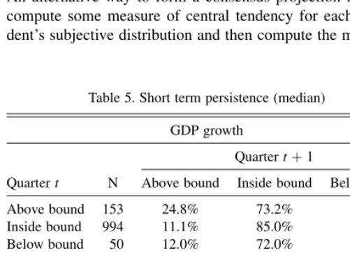
The SPF attaches an ID number to each forecaster, so we are able to analyze the behavior of individual forecasters across time. Table 5 compares forecasts in adjacent quarters. The table
Table 2. Upper bounds on mean/median/mode point predictions
GDP growth
Prediction Quarter 1 Quarter 2 Quarter 3 Quarter 4
Mean 83.01% 82.09% 88.89% 93.72%
Median 75.34% 77.44% 87.68% 89.86%
Mode 85.21% 86.74% 89.86% 92.03%
Inflation
Prediction Quarter 1 Quarter 2 Quarter 3 Quarter 4
Mean 82.42% 84.22% 84.30% 88.89%
Median 79.25% 82.29% 84.81% 87.63%
Mode 84.44% 85.68% 87.09% 89.90%
Table 3. Percent of forecasters using N intervals or less
GDP growth
1 2 3 4 5 6 7 8 9 10
Quarter 1 .0% 6.9% 32.3% 54.0% 71.8% 81.9% 90.4% 92.9% 95.1% 100.0%
Quarter 2 .5% 15.1% 43.5% 62.1% 78.1% 85.1% 90.0% 93.5% 95.4% 100.0%
Quarter 3 1.9% 22.9% 62.3% 77.0% 86.2% 90.3% 94.2% 96.1% 96.8% 100.0%
Quarter 4 11.1% 58.9% 82.6% 91.1% 94.7% 96.1% 97.3% 97.8% 98.5% 100.0%
Inflation
1 2 3 4 5 6 7 8 9 10
Quarter 1 .6% 15.0% 51.0% 74.1% 86.5% 91.9% 97.1% 97.4% 98.0% 100.0%
Quarter 2 1.7% 21.9% 55.4% 74.8% 85.7% 92.2% 94.9% 96.6% 98.3% 100.0%
Quarter 3 4.1% 33.4% 70.1% 84.1% 92.7% 94.9% 97.7% 98.0% 98.7% 100.0%
Quarter 4 14.7% 59.6% 84.6% 94.7% 97.0% 97.7% 98.7% 99.0% 99.0% 100.0%
considers point predictions in relation to the bounds for the median; the results for the mean and mode are similar and are omitted for brevity. Table 6 compares forecasts in Quarter t
with those made one, two, and three years later; that is, in Quarterstþ4k,k¼1, 2, 3.
The tables show evidence of both short- and long-run positive persistence in the relationship between point and probabilistic forecasts. A forecaster whose point prediction for inflation (GDP growth) lies above the upper bound for his mean/median/ mode one period is more likely to provide a point prediction above the upper bound for his mean/median/mode in later periods than is a forecaster whose point prediction is within or below the bounds for his mean/median/mode. This persistence is also found for forecasters whose point predictions lie below the lower bound for their means/medians/modes.
3.5 Consensus Projections
In its quarterly summary of new SPF findings, the Phila-delphia Fed makes considerable use of consensus projections, which are the median point predictions of the SPF respondents. An alternative way to form a consensus projection is to first compute some measure of central tendency for each respon-dent’s subjective distribution and then compute the median of
this measure across respondents. A particularly simple and appealing approach is to measure the central tendency of a sub-jective distribution by the midpoint of the interval in which the subjective median lies. As discussed previously, the SPF prob-abilistic forecasts always place the subjective median within an interval of width 0.01. Hence, a respondent’s subjective median must lie within 0.005 of the midpoint of this interval.
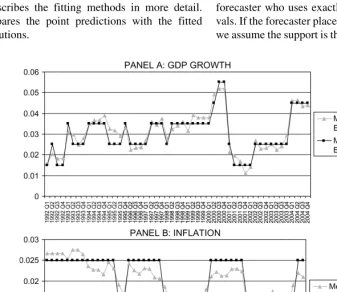
Figure 1 compares the standard consensus projections with this alternative for the period 1992–2004. We caution the reader that the Y-axes of the two panels of the figure have different scales, with the top panel running from 0 to 0.06 for GDP growth and the bottom one running from 0 to 0.03 for inflation. The different scales are necessitated by the fact that the GDP predictions are much more volatile than the inflation ones. Observe that the projections based on subjective medians always take one of the values 0.015, 0.025, 0.035, 0.045, or 0.055. This is so because the SPF intervals have midpoints at 0.005, 0.015, 0.025, and so on.
The figure illustrates well the two primary findings of our analysis. First, the standard and alternative consensus projec-tions tend to be quite close to one another and have the same qualitative time series variation. Indeed, the average absolute deviation between the two is only 0.0026 in the case of GDP growth and 0.0024 in the case of inflation. Second, to the extent that the two time series differ, the standard consensus projec-tion tends to give a slightly more favorable view of the econ-omy than does the alternative. On average, the standard consensus projection for GDP growth is 0.0006 above the alternative forecast. On average, the standard consensus pro-jection for inflation is 0.0010 below the alternative forecast.
4. PARAMETRIC ANALYSIS
The analysis of Section 3 has the great advantage of using the SPF data alone, without any assumptions about the shapes of forecasters’ subjective distributions for GDP growth and inflation. The accompanying disadvantage is that we can draw only limited conclusions about the relationship of point pre-dictions to probabilistic beliefs. Imposing assumptions enables sharper empirical analysis, albeit subject to the credibility of the assumptions imposed.
In this section, we report a parametric analysis whose most basic assumption is that probabilistic beliefs are unimodal. When an SPF probabilistic forecast assigns positive probability to three or more intervals, we furthermore assume that the subjective distribution is a member of the generalized Beta family and use the data to fit the Beta parameters. The gener-alized Beta distribution, which uses two parameters to describe the shape of beliefs and two more to give their support, is a flexible form that permits a distribution to have different values for its mean, median, and mode.
It is possible to fit a unique Beta distribution to the SPF data only when a forecast assigns positive probability to at least three intervals. This occurs in 2,234 of the 3,173 forecasts that we observe. The remaining 939 forecasts only assign positive probability to one or to two intervals. In these cases, we assume instead that the subjective distribution has the shape of an isosceles triangle whose base includes all of the intervals with greater probability mass and part of the other interval, if there
Table 4. Evidence of favorable point predictions
GDP growth
N Above bound Below bound
Mean 211 73.46% 26.54%
Median 280 73.93% 26.07%
Mode 186 58.60% 41.40%
Inflation
N Above bound Below bound
Mean 232 6.47% 93.53%
Median 254 22.44% 77.56%
Mode 204 12.25% 87.75%
Table 5. Short term persistence (median)
GDP growth
Quartert N
Quartertþ1
Above bound Inside bound Below bound
Above bound 153 24.8% 73.2% 2.0%
Inside bound 994 11.1% 85.0% 3.9%
Below bound 50 12.0% 72.0% 16.0%
Inflation
Quartert N
Quartertþ1
Above bound Inside bound Below bound
Above bound 50 10.0% 86.0% 4.0%
Inside bound 949 3.8% 86.5% 9.7%
Below bound 127 0.8% 70.1% 29.1%
is one. (In all cases with two intervals, the two are adjacent to one another and the majority of the probability mass lies in a bounded interval.) This assumption gives one parameter to be fit, which fixes the center and height of the triangle. An isos-celes triangle is symmetric, so the mean, median, and mode of the fitted subjective distribution necessarily coincide in these cases. This feature of the fit is not much of a practical concern, because the actual means, medians, and modes of forecasts that lie entirely within one or two intervals must lie relatively close to one another in any event.
Section 4.1 describes the fitting methods in more detail. Section 4.2 compares the point predictions with the fitted probability distributions.
4.1 Fitting Methods
4.1.1 Case 1—The Forecaster Uses 1 Bounded
Inter-val. We assume that the subjective distribution takes the shape of an isosceles triangle whose support is the interval. For ex-ample, if a forecaster places all probability in the interval [3%, 4%], we assume that the support of his distribution is [0.03, 0.04]. Then the base of the triangle has its center at 0.035 and has length 0.01. The height of the triangle is 200, yielding area equal to 1.
4.2.2 Case 2—The Forecaster Uses 2 Intervals. Every forecaster who uses exactly two intervals uses adjacent inter-vals. If the forecaster places equal probability in these intervals, we assume the support is the union of the intervals and we fit an
Table 6. Long-term persistence (median)
GDP growth
Quartert
Quartertþ4 Quartertþ8 Quartertþ12
N Above Inside Below N Above Inside Below N Above Inside Below
Above bound 116 25.0% 71.6% 3.4% 92 17.4% 78.3% 4.3% 81 19.8% 77.8% 2.5%
Inside bound 874 11.3% 86.2% 2.5% 678 12.1% 85.0% 2.9% 534 12.2% 84.3% 3.6%
Below bound 44 6.8% 79.5% 13.6% 35 17.1% 77.1% 5.7% 24 16.7% 79.2% 4.2%
Inflation
Quartert
Quartertþ4 Quartertþ8 Quartertþ12
N Above Inside Below N Above Inside Below N Above Inside Below
Above bound 34 5.9% 88.2% 5.9% 32 6.3% 87.5% 6.3% 28 7.1% 85.7% 7.1%
Inside bound 825 4.6% 85.2% 10.2% 635 4.9% 87.4% 7.7% 516 5.0% 86.4% 8.5%
Below bound 103 2.9% 76.7% 20.4% 88 4.5% 76.1% 19.3% 58 1.7% 82.8% 15.5%
Figure 1. Consensus projections using point and density forecasts.
isosceles triangle whose base has length 0.02 and whose height is 100. If a forecaster places more probability in one interval than the other, we assume that the support of the subjective distribution contains the entirety of the more probable interval. This restricts one endpoint of the support. With this restriction and our assumption that the subjective distribution is an isos-celes triangle, we are able to completely specify the dis-tribution: Suppose that a forecaster places probability a and
1ain the intervals [y%, (yþ1)%) and [(yþ1)%, (yþ2)%)
respectively, where a< 1
2. Letting t¼ straightforward to show that the isosceles triangle with height 200=ðtþ1Þand endpoints (yþ1t)% and (yþ2)% defines a subjective probability density function that is consistent with the respondent’s beliefs. Figure 2 illustrates our construction.
4.2.3 Case 3—The Forecaster Uses 3 or More
Inter-vals. In general, the probabilities that a forecaster reports for the 10 intervals in an SPF forecast reveal points on the cumulative distribution function (CDF) of his beliefs. For ex-ample, if a forecaster reports a 0.3 chance that GDP growth will be in the interval [2%, 3%), a 0.6 chance for the interval [3%, 4%), and a 0.1 chance for the interval [4%, 5%), we can infer these points on the forecaster’s CDF: F(0.02)¼0, F(0.03)¼
0.3, F(0.04)¼0.9, and F(0.05)¼1. When the forecast places positive probability on three or more intervals, we fit a unim-odal generalized Beta distribution to the data. The generalized Beta distribution has this CDF:
Betaðt;a;b;l;rÞ ¼
a1exdx. We choose a generalized Beta distribution,
because the two shape parametersa and b give considerable flexibility and the two location parameterslandrallow us to specify the support of the distribution. (The standard Beta distribution assumes that the support is the interval [0, 1].) To enforce unimodality, we maintain the restriction that a > 1 andb> 1.
Consider a forecaster whose observed points on his CDF are
F(t1),. . .,F(t10), wheret1,. . .,t10are the right endpoints of the
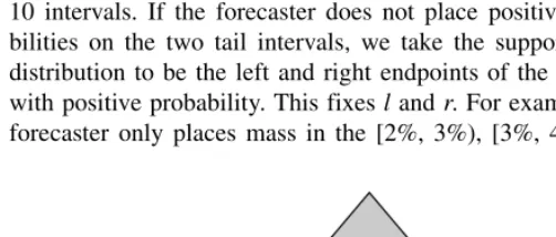
10 intervals. If the forecaster does not place positive proba-bilities on the two tail intervals, we take the support of the distribution to be the left and right endpoints of the intervals with positive probability. This fixeslandr. For example, if a forecaster only places mass in the [2%, 3%), [3%, 4%), and
[4%, 5%) intervals, then l ¼ 0.02 and r ¼ 0.05. We then minimize over the shape parametersaandb:
min
When a forecaster places mass in the lower tail interval, which is unbounded from below, we letlbe a free parameter in the minimization. Likewise, if a forecaster places mass in the upper tail, we letrbe a free parameter in the minimization. However, we restrict the support parameterslandrto lie within the most extreme values that have actually occurred in the United States since 1930. Thus, for change in GDP, we restrictl
andrto the range0.13 <l<r< 0.19. For inflation, we restrict
landr to the range0.12 < l< r< 0.12. For example, if a forecaster reports a 0.3 chance that GDP growth will be in the interval [4%, 5%], a 0.6 chance for the interval [5%, 6%], and a 0.1 chance for the interval [6%,‘%), the minimization
prob-lem becomes
4.2. Comparing the Point Predictions with the Fitted Probability Distributions
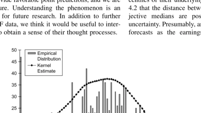
Having fitted a CDF to each SPF probabilistic forecast, we can compare the point predictions with the fitted CDFs. This is accomplished in Figures 3 and 4, the former for GDP growth and the latter for inflation. Figure 3 shows that forecasters tend to report point predictions for GDP growth that are high per-centiles of the fitted probability distributions. In contrast, Figure 4 shows that most forecasters report point predictions for inflation that are low percentiles. Overall, 41.16% of point predictions were equal to or below their fitted medians for the GDP growth questions, while 71.16% of point predictions were equal to or below their fitted medians for the inflation ques-tions. These results corroborate our earlier nonparametric finding, discussed in Section 3.3, that forecasters tend to pro-vide favorable point predictions relative to their probabilistic beliefs.
Moreover, we find that the distance between the point pre-diction and measures of central tendency are positively corre-lated with forecaster uncertainty. Letting DIST be the distance between a forecaster’s point prediction and his fitted median and IQR be the interquartile range of the fitted distribution, the correlation between DIST and IQR is 0.25 in the GDP growth case and 0.29 in the inflation case. This correlation seems reasonable if forecasters are giving favorable percentiles of their subjective distributions as point predictions; for example, if a forecaster always gave the 90th percentile of his dis-tribution as a point prediction, the distance between this point prediction and a measure of central tendency will shrink as the distribution tightens.
In Section 3.4, we showed nonparametrically that SPF forecasters exhibit some time series persistence, with those who give favorable point predictions in one quarter tending to do the same in subsequent quarters. Table 7 examines
Figure 2. Illustration of two interval cases.
persistence parametrically, by calculating the serial correlation of the point-forecast percentiles. We find considerable short-term persistence but less long-short-term persistence, especially in the inflation forecasts.
5. CONCLUSION
If people think probabilistically, as economists generally assume, their point predictions should somehow be related to their underlying subjective distributions. We have shown that most SPF point predictions are within 0.01 of forecasters’ sub-jective means/medians/modes. We have also shown that the deviations between point predictions and these measures of central tendency tend to be asymmetric, with point predictions tending to give a more favorable view of the economy than do subjective means/medians/modes. We do not know why fore-casters tend to provide favorable point predictions, and we are loathe to conjecture. Understanding the phenomenon is an important subject for future research. In addition to further analysis of the SPF data, we think it would be useful to inter-view forecasters to obtain a sense of their thought processes.
Whatever the reasons for forecaster behavior, our empirical findings have implications for research relying on point pre-dictions. For example, the accounting literature has docu-mented a positive relationship between the optimism of analysts’ earnings forecasts and the forecast horizon; Ramnath, Rock, and Shane (2006) review these findings. In particular, longer horizon earnings forecasts tend to be higher than the realized earnings, but the bias disappears for shorter horizon forecasts; in fact, there is some evidence that short horizon forecasts are slightly pessimistic. Some authors, for example, Richardson, Teoh, and Wysocki (2004), have argued that the observed pattern of bias reflects firms’ efforts to ‘‘guide’’ analysts’ forecasts down to beatable levels as the horizon shortens. Our findings suggest another explanation. It could be that analysts have rational expectations with respect to future earnings but that their point predictions are simply high per-centiles of their underlying distributions. Recall from Section 4.2 that the distance between SPF point predictions and sub-jective medians are positively correlated with forecaster uncertainty. Presumably, analysts become more certain of their forecasts as the earnings announcement date approaches.
Figure 4. Empirical distribution of point-forecast percentiles (inflation). Figure 3. Empirical distribution of point-forecast percentiles (GDP growth).
Hence, we should expect to find the positive relationship between point prediction optimism and forecast horizon that is documented in the accounting literature.
Our findings also have important implications outside aca-demia. It is standard practice for experts to give point pre-dictions. These point predictions may have significant consequences: the Congressional Budget Office’s (CBO’s) (www.cbo.gov) point predictions for the costs of legislative bills may affect legislators’ voting decisions, and financial analysts’ earnings forecasts and price targets may affect peo-ple’s investment decisions. The SPF evidence suggests that point predictions may have a systematic, favorable bias. This, plus the inescapable fact that point predictions reveal nothing about the uncertainty that forecasters feel, suggests that the agencies who commission forecasts should not ask for point predictions. Instead, they should elicit probabilistic expect-ations and derive measures of central tendency and uncertainty. This paper has shown how to derive measures of central tendency from the SPF probabilistic forecasts, both nonpara-metrically and paranonpara-metrically. The approaches developed in Sections 3 and 4 can also be applied to derive measures of uncertainty. An earlier working-paper version of this paper presents some preliminary analysis (Engelberg et al. 2006). Carrying that work forward is an important topic for future research.
APPENDIX: ROBUSTNESS CHECK: ROUNDING
Most probabilistic forecasts reported in the SPF are multiples of 0.05. This suggests that forecasters tend to round their responses. This phenomenon has also been documented by D’Amico and Orphanides (2006).
Rounding is common in surveys that elicit probabilistic expectations. Manski (2004) observes that, when respondents are asked for the ‘‘percent chance’’ that an event will occur, they tend to report values at 1% intervals at the extremes (i.e., 0, 1, 2 and 98, 99, 100) and at 5% intervals elsewhere (i.e., 5, 10,. . ., 90, 95). Of course, rounding is not unique to reports of probabilistic expectations—SPF forecasters and other survey respondents may round their point predictions as well. How-ever, we focus on rounding of the probabilistic forecasts here and take the point predictions at face value.
This appendix considers how rounding of the probabilistic forecasts may affect the findings presented in Tables 2 and 4.
There we showed the tendency for favorable point predictions in those cases in which point predictions are inconsistent with the means/medians/modes of forecasters’ subjective proba-bility distributions. We take possible rounding into account by splitting our observations into two cases.
A.1 Case 1—In Each Bin of a Given Forecast, the Forecaster’s Probability Mass is a Multiple of .05
In this case, we assume that the forecaster is rounding to multiples of .05. We do not know whether the forecaster is rounding up or rounding down, so we create two scenarios: the ROUND-UP scenario and the ROUND-DOWN scenario. In the ROUND-UP scenario, we take 0.05 of the probability mass from each bin used by the forecaster and move it to the next higher bin. The result is that 0.05 of mass is subtracted from the lowest bin used and placed in the bin that is immediately above the highest bin used. (When the highest bin is adjacent to the right-hand tail bin, we form a new adjacent bin of width 0.01 within the right-hand tail and place the mass there. When the highest bin is the right-hand tail bin, 0.05 is added to this bin.) In the ROUND-DOWN scenario, we similarly take 0.05 of the probability mass from each bin used by the forecaster and move it to the next lower bin.
For example, suppose that a forecaster places 0.65 probability mass in the 2–3% bin and 0.35 in the 3–4% bin. The ROUND-UP scenario would put 0.60 in the 2–3% bin, 0.35 in the 3–4%
Table 7. Persistence of point-forecast percentiles
GDP growth
Quartert
Quartertþ1 Quartertþ4 Quartertþ8 Quartertþ12
N Correlation N Correlation N Correlation N Correlation
Point-forecast percentile 1,197 0.2553 1,034 0.0847 805 0.1196 639 0.1490
Inflation
Quartert
Quartertþ1 Quartertþ4 Quartertþ8 Quartertþ12
N Correlation N Correlation N Correlation N Correlation
Point-forecast percentile 1,126 0.2157 962 0.0496 755 0.0243 602 0.0144
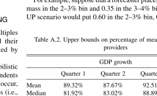
Table A.2. Upper bounds on percentage of mean/median/mode providers
GDP growth
Quarter 1 Quarter 2 Quarter 3 Quarter 4
Mean 89.32% 87.67% 92.51% 95.65%
Median 81.92% 83.02% 88.89% 92.27%
Mode 85.48% 86.74% 89.86% 92.03%
Inflation
Quarter 1 Quarter 2 Quarter 3 Quarter 4
Mean 88.18% 90.29% 89.37% 92.42%
Median 84.44% 85.44% 88.10% 90.15%
Mode 85.01% 85.92% 87.09% 89.90%
bin, and 0.05 in the 4–5% bin. The ROUND-DOWN scenario would put 0.05 in the 1–2% bin, 0.65 in the 2–3% bin, and 0.30 in the 3–4% bin. These two scenarios bound the forecaster’s true beliefs under the assumption that (1) the forecaster rounds to a multiple of 0.05 when giving his forecasts and (2) the true support of his subjective probability distribution does not extend more than 1% in either direction beyond his expressed beliefs.
A.2 Case 2—In at Least One Bin of a Given Forecast, the Forecaster’s Probability Mass is not a
Multiple of 0.05
In this case, we assume the forecaster is not rounding to a multiple of 0.05 and we do not adjust his responses.
Of all the inflation forecasts, 84% were in the case 1 cat-egory and 16% were case 2. Of the GDP forecasts, 78% were in the case 1 category and 22% were case 2.
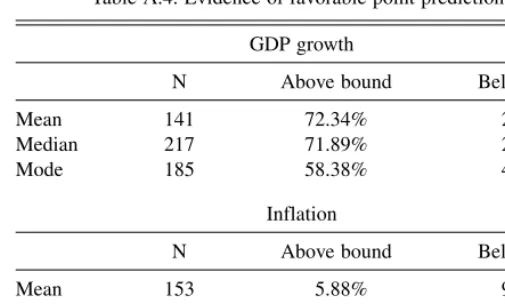
We now recompute the bounds on the mean, median, and mode and reproduce Tables 2 and 4 from the text. When an observation falls into case 1, the bounds on the mean neces-sarily widen, provided that they are not already infinite. Depending on the particular distribution, the bounds on the median and mode may or may not widen. When an observation falls into case 2, the bounds do not change. Comparison of Tables 2 and 4 with their revised versions shows that attention to the possibility of rounding does not change the qualitative findings reported earlier.
ACKNOWLEDGMENTS
The authors thank the editor, the associate editor, an anon-ymous referee, Ravi Jagannathan, and Zhiguo He for helpful
comments. We have benefitted from the opportunity to present this work at a March 2006 conference on economic expect-ations in Madrid and in a seminar at the Federal Reserve Bank of New York. We also thank Tom Stark of the Federal Reserve Bank of Philadelphia for his help with the data.
[Received September 2006. Revised June 2007.]
REFERENCES
Brenner, M., and Landskroner, Y. (1983), ‘‘Inflation Uncertainties and Returns on Bonds,’’Economica, 50, 463–468.
Capistran, C., and Timmermann, A. (2006), ‘‘Disagreement and Biases in Inflation Expectations,’’ Department of Economics, University of California at San Diego.
Clements, M. (2007), ‘‘Internal Consistency of Survey Respondents’ Forecasts: Evidence Based on the Survey of Professional Forecasters,’’ Department of Economics, University of Warwick.
Cukierman, A., and Wachtel, P. (1979), ‘‘Differential Inflationary Expectations and the Variability of the Rate of Inflation: Theory and Evidence,’’The American Economic Review, 69, 595–609.
D’Amico, S., and Orphanides, A. (2006), Uncertainty and disagreement in economic forecasting. Board of Governors of the Federal Reserve System. Diether, K. B., Malloy, C. J., and Scherbina, A. (2002), ‘‘Differences of
Opinion and the Cross Section of Stock Returns,’’The Journal of Finance,
57, 2113–2141.
Engelberg, J., Manski, C., and Williams, J. (2006), ‘‘Comparing the Point Predictions and Subjective Probability Distributions of Professional Fore-casters,’’ National Bureau of Economic Research Working Paper W11978. Giordani, P., and Soderlind, P. (2003), ‘‘Inflation Forecast Uncertainty,’’
European Economic Review, 47, 1037–1059.
Hahm, J.-H., and Steigerwald, D. (1999), ‘‘Consumption Adjustment under Time-Varying Income Uncertainty,’’ The Review of Economics and Sta-tistics, 81, 32–40.
Hayford, M. (2000), ‘‘Inflation Uncertainty, Unemployment Uncertainty, and Economic Activity,’’Journal of Macroeconomics,22, 315–329.
Juster, T. (1966), ‘‘Consumer Buying Intentions and Purchase Probability: An Experiment in Survey Design,’’Journal of the American Statistical Associ-ation, 61, 658–696.
Levi, M., and Makin, J. H. (1979), ‘‘Fisher, Phillips, Friedman and the Mea-sured Impact of Inflation on Interest,’’The Journal of Finance, 34 (1), 35–52. ——— (1980), ‘‘Inflation Uncertainty and the Phillips Curve: Some Empirical
Evidence,’’The American Economic Review, 70 (5), 1022–1027.
Makin, J. (1982), ‘‘Anticipated Money, Inflation Uncertainty, and Real Eco-nomic Activity,’’The Review of Economics and Statistics, 64, 126–134. Mankiw, N. G., Reis, R., and Wolfers, J. (2003), ‘‘Disagreement about Inflation
Expectations,’’NBER Macroeconomics Annual 2003, Cambridge, MA: MIT Press.
Manski, C. F. (2004), ‘‘Measuring Expectations,’’Econometrica, 72, 1329– 1376.
——— (1990), ‘‘The Use of Intentions Data to Predict Behavior: A Best Case Analysis,’’Journal of the American Statistical Association, 85 (412), 934– 940.
Ramnath, S., Rock, S., and Shane, P. (2006), ‘‘A Review of Research Related to Financial Analysts’ Forecasts and Stock Recommendations,’’ Leeds School of Business, University of Colorado at Boulder.
Richardson, S., Teoh, S. H., and Wysocki, P. (2004), ‘‘The Walkdown to Beatable Analyst Forecasts: The Role of Equity Issuance and Insider Trading Incentives,’’Contemporary Accounting Research, 21 (4), 885–924. Zarnowitz, V., and Lambros, L. A. (1987), ‘‘Consensus and Uncertainty in
Economic Prediction,’’The Journal of Political Economy, 95 (3), 591–621.
Table A.4. Evidence of favorable point predictions
GDP growth
N Above bound Below bound
Mean 141 72.34% 27.66%
Median 217 71.89% 28.11%
Mode 185 58.38% 41.62%
Inflation
N Above bound Below bound
Mean 153 5.88% 94.12%
Median 200 11.50% 88.50%
Mode 201 11.44% 88.56%