Planar Graphs as Minimal Resolutions of
Trivariate Monomial Ideals
Ezra Miller
Received: May 4, 2001 Revised: March 11, 2002
Communicated by G¨unter M. Ziegler
Abstract. We introduce the notion of rigid embedding in a grid surface, a new kind of plane drawing for simple triconnected planar graphs. Rigid embeddings provide methods to (1) find well-structured (cellular, here) minimal free resolutions for arbitrary monomial ideals in three variables; (2) strengthen the Brightwell–Trotter bound on the order dimension of triconnected planar maps by giving a geometric reformulation; and (3) generalize Schnyder’s angle coloring of planar triangulations to arbitrary triconnected planar maps via geometry. The notion of rigid embedding is stable under duality for planar maps, and has certain uniqueness properties.
2000 Mathematics Subject Classification: 05C10, 13D02, 06A07, 13F55, 68R10, 52Cxx
Keywords and Phrases: planar graph, monomial ideal, free resolution, order dimension, (rigid) geodesic embedding
Contents
Introduction and summary 44
I Geodesic embedding in grid surfaces 49
1 Planar maps 49
2 Grid surfaces 51
4 Contracting rigid geodesics 57 5 Triconnectivity and rigid embedding 66
II Monomial ideals 68
6 Betti numbers 68
7 Cellular resolutions 69
8 Graphs to minimal resolutions 70
9 Uniqueness vs. nonplanarity 72
10 Deformation and genericity 73
11 Ideals to graphs: algorithm 75
12 Ideals to graphs: proof 77
III Planar maps revisited 80
13 Orthogonal coloring 80
14 Orthogonal flows 81
15 Duality for geodesic embeddings 84
16 Open problems 86
Introduction
Simple triconnected planar graphs admit numerous characterizations. Two famous examples include Steinitz’ theorem on the edge graphs of 3-polytopes, and the Koebe–Andreev–Thurston circle packing theorem (see [Zie95] for both). These results produce “correct” planar (or spherical) drawings of the graphs in question, from which a great deal of geometric and combinatorial information flows readily.
This paper introduces a new kind of plane drawing for simple triconnected pla-nar graphs, from which a great deal ofalgebraicand combinatorial information flows readily. Thesegeodesic embeddingsinsidegrid surfacesprovide methods to
• strengthen the Brightwell–Trotter bound on the order dimension of tri-connected planar maps [BT93] by giving a geometric reformulation; and
• generalize Schnyder’s angle coloring for planar triangulations [Tro92, Chapter 6] to arbitrary triconnected planar maps via geometry.
We note that Felsner’s generalization of Schnyder’s angle coloring [Fel01] co-incides with theorthogonal colorings independently discovered here as conse-quences of geometric considerations. In parallel with circle-packed and polyhe-dral graph drawings, additional evidence for the naturality of geodesic embed-dings comes from their stability under duality, and the uniqueness properties enjoyed by “correct” geodesic embeddings—called rigid embeddings in what follows—for a given planar map.
The plan of the paper is as follows. Immediately following this Introduction is a section containing two theorems summarizing the equivalences and construc-tions forming main results of the paper. After that, the paper is divided into three Parts.
Part I lays the groundwork for geodesic and rigid embeddings in grid surfaces, and is geared almost entirely toward proving Theorem 5.1: the rigid embedding theorem. Terminology for the rest of the paper is set in Section 1, which also states a standard criterion for triconnectivity under edge contraction that serves as an inductive tool in the proof of Theorem 5.1. Then Section 2 presents the definition of grid surfaces, as well as the vertex and edge axioms for geodesic and rigid embeddings. Their consequences, the region and rigid region axioms, appear in Propositions 2.3 and 2.4. The first connection with order dimension comes in Corollary 2.5.
Sections 3 and 4 consist of stepping stones to the rigid embedding theorem. The basic inductive step for abstract planar maps is Lemma 3.1, which motivates the preliminary grid surface construction of Lemma 3.2. Induction for grid surfaces occupies the three Propositions in Section 4. They have been worded so that their rather technical proofs (particularly that of Proposition 4.2) may be skipped the first time through; instead, the Figures should provide ample intuition.
Section 5 completes the induction with a few more arguments about abstract planar maps. Corollary 5.2 recovers the Brightwell–Trotter bound on order dimension from rigid embedding.
The focus shifts in Part II to the algebra of monomial ideals in three variables, specifically their minimal free resolutions. A review of the standard tools oc-cupies Section 6, while Section 7 recaps the more recent theory of cellular resolutions, along with a triconnectivity result (Proposition 7.2) suited to the applications here. Theorem 8.4 says how geodesic embeddings become min-imal free resolutions. Corollary 8.5 then characterizes triconnectivity as the condition guaranteeing that a planar map supports a minimal free resolution of some artinian monomial ideal.
(Corol-lary 9.1), which implies in particular that every minimal cellular resolution of the corresponding monomial ideal is planar. Surprisingly, there can exist non-planar cell complexes supporting minimal free resolutions of trivariate artinian monomial ideals that are sufficiently nonrigid; Example 9.2 illustrates one. Sections 10–12 are devoted to producing minimal cellular free resolutions of ar-bitrary monomial ideals in three variables (Theorem 11.1). The deformations reviewed in Section 10 serve as part of the algorithmic solution pseudocoded in Algorithm 11.2. The proof of correctness for the algorithm and the theorem, which occupy Section 12, are rather technical and delicate. As with Section 4, the pictures may give a better feeling for the methods than the proofs them-selves, at least upon first reading.
Part III continues where Part I left off, with more combinatorial theory for pla-nar maps. Section 13 introduces orthogonal coloring, which generalizes Schny-der’s angle coloring and abstracts the notion of geodesic embedding (Propo-sition 13.1). Then, Section 14 shows how orthogonal coloring encodes the abstract versions of the orthogonal flows that played crucial roles in Section 2. As a consequence, Proposition 14.2 shows that orthogonal flows are examples of—but somewhat better than—normal families of paths, connecting once again with the work of Brightwell and Trotter on order dimension. Section 15 demon-strates how Alexander duality for grid surfaces (or monomial ideals) manifests itself as duality for planar maps geodesically embedded in grid surfaces. Finally, Section 16 presents some open problems related to the notions devel-oped in earlier sections, including a conjecture on orthogonal colorings and some problems on classifying cell complexes supporting minimal resolutions. Further questions concern applications of the present results to broader com-binatorial algebraic problems, notably how to describe the “moduli space” of all minimal free (or injective) resolutions of ideals generated by a fixed number of monomials.
After completing an earlier version of this paper, the author was informed that Stefan Felsner had independently discovered the theory in Sections 13 and 14 [Fel01, Sections 1 and 2]. In addition, Felsner proved Conjecture 16.3 in [Fel02] after reading the preliminary version of this paper. See Section 16.3 for details and consequences.
Part III is almost logically independent of Part II, the only exceptions being Lemmas 8.2 and 8.3. Thus, the reader interested primarily in the combinatorics of planar graphs (as opposed to resolutions of monomial ideals) can read Parts I and III, safely skipping everything in Part II except for these two lemmas. The reader interested primarily in resolutions of monomial ideals should skip everything in Sections 3–5 except for the statement of Theorem 5.1.
Acknowledgements
proof. The Alfred P. Sloan Foundation and the National Science Foundation funded various stages of this project.
Summary theorems
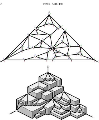
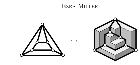
For the sake of perspective and completeness, we collect the main ideas of the paper into a pair of precisely stated summary theorems. Their proofs are included, in the sense that the appropriate results from later on are cited. All of the notions appearing in Theorems A and B will be introduced formally in due time; until then, brief descriptions along with Figure 1 should suffice. Let M be a connected simple planar map—that is, a graph embedded in a surfaceShomeomorhpic to the planeR2. All graphs in this paper have finitely many vertices and edges. Fix a point∞ ∈Sfar fromM, and define the exterior region of M to be the connected component ofSrM containing∞. Given three vertices ˙x,y,˙ z˙∈M bordering the exterior region, form the extended map
M∞( ˙x,y,˙ z˙) by connecting ˙x,y,˙ z˙ to∞. Call a graph triconnected either if it is a triangle, or if it has at least four vertices of which deleting any pair along with their incident edges leaves a connected graph. A set of paths leaving a fixed vertexν ∈M is said to be independent if their pairwise intersection is{ν}. Letk[x, y, z] be the polynomial ring in three variables over a fieldk, and letI⊂ k[x, y, z] be an ideal generated by monomials. The grid surfaceScorresponding toIis the boundary of the staircase diagram ofI, which is drawn (as usual) as the stack of cubes corresponding to monomials not in I. Rigid embedding of a planar map M in S involves identifying the edges ofM as certain piecewise linear geodesics inS, and constitutes an inclusion of the vertex-edge-face poset of M into N3. Orthogonal coloringM involves coloring the angles in M with three colors according to certain rules. Since it would take too long to do real justice to the definitions of ‘rigid embedding’ and ‘orthogonal coloring’ here, Figure 1 will have to do for now. The outer corners in the orthogonal coloring and the vectors on the axes inS are called axial vertices. The grid surface S
is called axial when Iis artinian.
SupposeM is a cell complex (finite CW complex) whose faces are labeled by vectors inN3, in such a way that the unionM¹αof faces whose labels precede
α∈ N3 is a subcomplex of M for every α. Roughly speaking, M supports a
cellular free resolution ofI if the boundary complex of M¹α with coefficients in kis theN3-degree αpiece of a free resolution of I, for every α∈N3.
Theorem A LetM be a planar map. The following are equivalent.
1. M has three vertices x,˙ y,˙ z˙ bordering its exterior region for which
M∞( ˙x,y,˙ z˙)is triconnected.
2. M has three vertices x,˙ y,˙ z˙ bordering its exterior region to which every vertex ofM has independent paths.
z
Figure 1: Orthogonal coloring and rigid embedding of an extended map
5. M supports a cellular minimal free resolution of some artinian monomial ideal ink[x, y, z].
Every artinian monomial ideal in k[x, y, z] has a minimal cellular resolution supported on a cell complex M satisfying these conditions; in fact, Algo-rithm 11.2 produces such anM automatically.
Proof. 4⇒3 follows from Proposition 13.1. 3 ⇒2 follows from Proposition 14.2. 2 ⇒1 follows easily from the definitions. 1 ⇒4 is Theorem 5.1.
The final statement comes from Theorem 11.1 and Proposition 12.4. ✷
Similar—but weaker—statements apply to minimal cellular free resolutions of arbitrary (not necessarily artinian) monomial ideals ink[x, y, z].
Theorem B Let N be a planar map. The following two conditions are equiv-alent.
1. N can be rigidly embedded in some grid surface.
2. N can be obtained by deletingx,˙ y,˙ z˙ and all edges incident to them from some planar mapM satisfying the equivalent conditions in Theorem A.
These conditions imply that
3. N supports a minimal free resolution of some monomial ideal ink[x, y, z]. Every monomial ideal in k[x, y, z] has a minimal free resolution supported on a planar map N satisfying conditions 1 and 2; such an N can be produced algorithmically.
Proof. 1⇒2 follows from Theorem 8.4 and Lemma 8.2. 2 ⇒1 follows from Theorem 5.1 and Lemma 8.2. 1 ⇒3 follows from Theorem 8.4.
The first half of the final statement is Theorem 11.1 along with the first para-graph of its proof on p. 80; add in Proposition 12.4 for the algorithmic part. ✷
In reality, the more detailed versions later on are considerably more precise, demonstrating how some of the equivalent descriptions naturally give rise to others.
Part I
Geodesic embedding in grid surfaces 1 Planar maps
LetV ={ν1, . . . , νr} be a finite set. AgraphGwith vertex setV is uniquely determined by a collectionE ⊆¡V2¢of edges, each consisting of a pair of vertices. Except for one paragraph at the beginning of Section 15, we consider only simple graphs—that is, without loops or multiple edges—so G is an abstract simplicial complex of dimension 1 having vertex setV. ThusGcan be regarded as a topological space, via any geometric realization.
LetSbe a surface homeomorphic to the Euclidean planeR2. Aplane drawing
of G in S is a continuous morphism G ֒→ S of topological spaces that is a homeomorphism onto its image. If G is connected, the image M is called a planar map. Deleting the images of the vertices and edges of G from S
are isomorphicif they result from plane drawings of the same graph G, their regions have the same boundaries in G, and the boundaries of their exterior regions correspond. We often blur the distinction between a planar map and the underlying graph, by not distinguishing a vertex (resp. edge) ofGfrom the corresponding point (resp. arc) ofM in the surfaceS.
A graphGisk-connectedeither ifGis the complete graph onkvertices, or if
G has at least k+ 1 vertices, and given any k−1 vertices ν1, . . . , νk−1 of G,
the deletion del(G;ν1, . . . , νk−1) is connected. Here, the deletion is obtained
by removingν1, . . . , νk−1 as well as all edges containing them fromG. In case k= 2 or 3, the graphGis called biconnectedortriconnected, respectively. Suppose thateis an edge of a planar mapM, and that none of the (one or two) regions containingeis a triangle. ThecontractionM/eofM alongeis obtained by removing the edgee and identifying the two vertices ofe. The underlying graph ofM/eis the topological quotientG/e; it is still simple becauseeis the only edge connecting its vertices in G(so G/ehas no loops) and no triangles contain e in G (so G/e has no multiple edges). Some plane drawing of M/e
is obtained by literally contracting the edge e in M (technically: there is a homotopyG×[0,1]→Ssuch thatG×t→S is a plane drawing ofGfort <1, whileG×1→Sis a compositionG→G/e→S with the second map being a plane drawing). Contraction will be a crucial inductive tool, via a well-known criterion for triconnectivity under contraction:
Proposition 1.1 Let M be a triconnected planar map with at least four ver-tices, and let ebe an edge. If there exist two regions F, F′ ofM such that
1. e∩F ande∩F′ are the two vertices of e, and 2. F∩F′ is nonempty,
then either e borders a triangle or the contraction M/e fails to be tricon-nected. Conversely, if e borders no triangles and M/e is triconnected, then no such F, F′ exist.
Thinking of the surface S∼=R2 as the 2-sphere minus ∞, many of the planar maps M in this paper result by embedding some graph G∞ in the sphere with ∞ as a vertex, and then considering the induced plane drawing M of del(G∞;∞). When this is the case, we frequently need to consider the subset
M∞ ⊂ S obtained by omitting the point ∞ from the plane drawing of G∞ in the sphere; thus some of the vertices inM connect to the missing point∞
by unbounded arcs in S. More generally, define an extended map M∞ ⊂S to be the union of a planar map M and a set of infinite nonintersecting arcs connecting some of its vertices to ∞. The closure M∞ of M∞ in the sphere need not be a simple graph because it can have doubled edges: some vertex in
M could have two or more unbounded arcs inM∞containing it.
(in order) proceeding counterclockwise around the exterior cycle. Having cho-sen axial vertices, define M∞( ˙x,y,˙ z˙) ⊂ S to be the union of M and three unbounded arcs, called thex,y, andz-axes, connecting ˙x,y,˙ z˙to∞. We some-times blur the distinction between M∞( ˙x,y,˙ z˙) and its closure M∞( ˙x,y,˙ z˙) in the sphere. For instance, we say thatM∞( ˙x,y,˙ z˙) is triconnected if the graph underlyingM∞( ˙x,y,˙ z˙) is.
2 Grid surfaces
Let Rdenote the real numbers. Write vectors in R3 as α= (α
x, αy, αz), and partially order R3 by setting α¹β (read ‘αprecedes β’) whenever α
u ≤βu for allu∈ {x, y, z}. Say that α∈R3 strongly precedesβ∈R3 whenα
u< βu for allu=x, y, z; this is stronger than sayingα≺β. (Throughout this paper, the letter u denotes any one of x, y, z, in the same way that xi denotes one ofx1, . . . , xn.) Useα∨βandα∧βto denote thejoin(componentwise maximum) andmeet(componentwise minimum) ofα, β∈R3.
LetV ⊂N3⊂R3 be a set of pairwise incomparable elements, whereNdenotes the set of nonnegative integers. The order filter
hVi = {α∈R3|αºν for someν∈ V}
generated by V is a closed subset of the topological space R3. Its boundary
SV is called agrid surfaceorstaircase. Orthogonal projection onto the plane
x+y+z= 0 restricts to a homeomorphismSV ∼=R2. (This homeomorphism gives the correspondence between rhombic tilings of the orthogonal projection of the |x| × |˙ y| × |˙ z|˙ parallelepiped and plane partitions of the |x| × |˙ y|˙ grid with parts at most |z|˙ . The grid surface in Figure 1 clearly demonstrates the homeomorphism: the diagram is, after all, drawn faithfully on the two-dimensional page.)
One of the basic properties of grid surfaces is thatα∈ SV wheneverρ, σ∈ SV and ρ¹α¹σ. Therefore, ifρ, σ ∈ SV andρ¹σ, thenSV contains the line segment inR3 connectingρto σ. In particular, if ν, ω ∈ V satisfyν∨ω ∈ SV, then SV contains the union [ν, ω] of the two line segments joiningν andω to
ν∨ω; we refer to such arcs as elbow geodesics1 in SV. Whenν andω are the only vectors inV precedingν∨ω, the arc [ν, ω] is called arigid geodesic. Denote the nonnegative rays of the coordinate axes inR3byX,Y, andZ, and use the letterU to refer to any ofX, Y, Z. The ray ν+U intersectsSV in an oriented line segment Uν called the orthogonal rayleaving ν in the direction of U. Thus every point inV has precisely three orthogonal rays, one parallel to each coordinate axis and all contained inSV, although some orthogonal rays may be unbounded while others are bounded.
If Uν is bounded, so it has an endpoint besides ν, then the other endpoint of Uν can always be expressed as a joinν∨ω for some ω ∈ V. When there is
1
Elbow geodesics do minimize length for the metric onSV induced by the usual metric
onR3
exactly one such pointω, so [ν, ω] is a rigid geodesic, we say thatνorUνpoints towardω.
Observe thatν∨ω must share two coordinates with at least one (and perhaps both) ofν andω, so every elbow geodesic contains at least one orthogonal ray. Making compatible choices of elbow geodesics containing all orthogonal rays yields a planar map. To be precise, a plane drawing M ֒→ SV is ageodesic grid surface embedding, or simply ageodesic embeddinginSV, if the following two axioms are satisfied:
(Vertex axiom) The vertices ofM coincide withV.
(Elbow geodesic axiom) Every edge of M is an elbow geodesic in SV, and every bounded orthogonal ray in SV is part of an edge ofM.
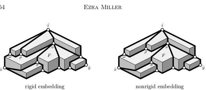
With the following stronger edge axiom instead,M ֒→ SV is arigid embedding, which we sometimes phrase by saying thatM isrigidly embeddedin SV:
(Rigid geodesic axiom) The elbow geodesic exiom holds, and every edge ofM is a rigid geodesic inSV.
The rigid geodesic axiom really consists of three parts, each of which puts nontrivial restrictions on SV or M: every bounded orthogonal ray in SV is part of a rigid geodesic (a priori, this has nothing to do withM); every rigid geodesic inSV is an edge ofM; and every edge ofM is a rigid geodesic inSV. Lemma 2.1 Let M ֒→ SV be a geodesic or rigid embedding. Suppose V is in order-preserving bijection with another set Ve of vertices via ν ↔ νe, so that
νu ≤ ωu ⇔ νeu ≤ eωu for all ν, ω ∈ V and u ∈ {x, y, z}. Then the elbow or rigid geodesics in SVe constitute another geodesic or rigid embedding of M.
In particular, linearly scaling one or more coordinate axes by integer factors preserves geodesic or rigid embeddings.
Proof. Purely order-theoretic properties ofV determine whether ν and ω are the endpoints of an elbow geodesic, or whetherν points towardω. ✷
Any geodesic embeddingM ֒→ SV determines an extended map
M∞ = M ∪(unbounded orthogonal rays). A special case occurs whenSV isaxial, having axial vectors
˙
x= (|x|,˙ 0,0), y˙ = (0,|y|,˙ 0), and z˙= (0,0,|z|˙)
in V for nonzero |x|,˙ |y|,˙ |z| ∈˙ N. Thus, if M is geodesically embedded in an axial grid surface SV, we can define the axial vertices of M to be the axial vectors inV, and setM∞( ˙x,y,˙ z˙) =M∪Xx˙∪Yy˙∪Zz˙. (Precisely two bounded
vertices ˙x,y,˙ z˙, then we require any geodesic embeddingM ֒→ SVto send these axial vertices to axial vectors inV.
Suppose M is geodesically embedded in the axial grid surfaceSV. The edge of M leaving any vertex ν 6= ˙z along the vertical orthogonal ray Zν con-nectsνto another vertexωwith strictly largerz-coordinate, but weakly smaller
xandy-coordinates. Continuing in this manner constructs anorthogonal flow [ν,z˙] from ν to ˙z that is increasing in z, but weakly decreasing in x and y. It follows that [ν,z˙] and the similarly constructed paths [ν,x˙] and [ν,y˙] are independent, meaning that they intersect pairwise only at ν itself. Since [ ˙x,y˙], [ ˙y,z˙], and [ ˙z,x˙] partition the exterior cycle of M into three arcs, the contractible sets bounded by
[ ˙x, ν,y˙] := [ν,x˙]∪[ν,y˙]∪[ ˙x,y˙]
and its cyclically permuted analogues partition the regions ofM.
Lemma 2.2 Suppose M ֒→ SV is an axial geodesic embedding, and ν ∈ V borders a region contained in [ ˙x, ω,y˙]. Then νz ≤ ωz, with strict inequality if ν 6∈ [ω,x˙]∪[ω,y˙]. A similar statement holds for arbitrary permutations of x, y, z.
Proof. The orthogonal flow [ν,z˙] must cross [ω,x˙] or [ω,y˙], atν′ ∈[ω,x˙], say. Concatenating the part of [ω,x˙] fromωtoν′ with the part of [ν,z˙] fromν′ toν yields a path from ω toν that is weakly decreasing inz. This path is strictly decreasing if ν 6∈[ω,x˙]∪[ω,y˙], for then it traverses (downwards) the vertical
orthogonal rayZν. ✷
Proposition 2.3 (Region axiom) LetM ֒→ SV be an axial geodesic embed-ding, andF a bounded region ofM. IfαF is the join of the vertices ofF, then
αF ∈ SV, and every vertex ν∈F shares precisely one coordinate with αF.
Proof. Ifω∈ V, then Lemma 2.2 implies there is someu∈ {x, y, z} such that
νu≤ωu for allν ∈F. This showsω cannot strongly precedeαF, soαF ∈ SV; every vertexν∈Ftherefore shares at least one coordinate withαF. Suppose by symmetry thatνz= (αF)z. The two edges ofF containingν cannot increase in z, so they exit ν counterclockwise of Xν and clockwise of Yν. At least one of these edges strictly increases in x, and another strictly increases in y,
completing the proof. ✷
rigid embedding nonrigid embedding
ρ
ρ
σ σ
ν ν
ω ω
˙ x ˙
x y˙ y˙
˙ z ˙
z
F F
Figure 2: The rigid region axiom and its failure for nonrigid embeddings
Proposition 2.4 (Rigid region axiom) Let M ֒→ SV be a rigid axial em-bedding, and F a region of M∞( ˙x,y,˙ z˙). IfαF is the join of the vertices of F andω∈ SV, thenω∈F ⇔ω¹αF.
Proof. The claim is obvious if F is one of the three unbounded regions, so assume F is bounded. Since ω ∈ F ⇒ ω ¹ αF by definition, let ω 6∈ F, and assume F is contained in [ ˙x, ω,y˙] by symmetry. Either ωz> νz for some vertex ν ∈F with maximal z-coordinateνz = (αF)z, in which case the proof is trivial, or all vertices ofF withz-coordinate (αF)z lie on [ω,x˙]∪[ω,y˙], by Lemma 2.2. Assume there is one on [ω,y˙] by transposingxandyif necessary, and letν∈F∩[ω,y˙] be closest toω.
The vertex ρ ∈[ω,y˙] pointing towardν has the samez-coordinate as ν (be-cause ωz ≥ρz ≥νz and ωz =νz), so the rigid geodesic [ρ, ν] consists of the orthogonal rays Yρ and Xν. Of ν’s two neighbors in F, let σ have smaller
y-coordinate. Since ρ6=σ and σ6∈ [ω,y˙], the edge connecting ν to σ exits ν
strictly counterclockwise of Xν and strictly clockwise of Yν. Thus σz < νz, whence σx = (αF)x by the region axiom (Proposition 2.3). But ρ6¹ν∨σby the rigid geodesic axiom, while ρz =νz = (ν∨σ)z and ρy < σy = (ν∨σ)y by construction. Therefore ρx >(ν∨σ)x =σx = (αF)x. The proof is complete
becauseω decreases in xalong [ω,y˙] to ρ. ✷
Corollary 2.5 Let M ֒→ SV be an axial rigid embedding. If P is a vertex, edge, or bounded region ofM, letαP denote join of the vertices inP. The map sending P 7→αP constitutes an embedding in N3 of the vertex-edge-face poset of M.
Proof. Immediate from the vertex, rigid geodesic, and rigid region axioms. ✷
3 Gluing geodesic embeddings
Let M be a planar map with axial vertices ˙x,y,˙ z˙ and extended mapM∞ =
M∞( ˙x,y,˙ z˙). Suppose C is a simple cycle inM having three counterclockwise ordered vertices ¨x,y,¨ z¨, and furthermore that C bounds a closed disk R ⊂S
that is a union of bounded regions in M. Following Brightwell and Trotter (cf. [Tro92, Chapter 6], although our definition differs slightly), we call C a ring if every edge ofM not contained inR intersectsR in a (possibly empty) subset of {x,¨ y,¨ z}¨ . The double-dotted vertices play the roles of axial vertices for a smaller map N = M ∩R “glued into” M by external edges emanating from N at ¨x,y,¨ z¨. Although we allow ¨ufor u∈ {x, y, z} to equal the original axial vertex ˙u∈M, we exclude the case whereCis the exterior cycle ofM by referring to aproper ring.
Assume for each u=x, y, zthat the vertex ¨umeets at least one edge in M∞ not contained inR(this occurs whenM∞is triconnected). If there are at least two such edges then set ¨u= ¨u. Otherwise, call the unique edgeeu¨ and name
its other endpoint ¨u. Here, ¨u= ∞ is allowed because ¨u = ˙u is; but if C is a proper ring, then at most one of ¨x,y,¨ ¨z can equal ∞, because there are no proper rings containing two axial vertices ˙u∈ {x,˙ y,˙ z}˙ such thatRcontains all of their edges inM. Indeed, it would be impossible to choose the third vertex ¨u
from the pair of last points on the exterior cycle ofM going from the two axial vertices onC toward the third.
The closure in the 2-sphere of the subsetM∞rRis a planar map whose inter-section withRequals{x,¨ y,¨ z}¨ . Construct thecontractionM∞/Rby leaving off the edges{eu¨ |u¨6= ¨u} as well as their endpoints ¨uonC, and then connecting
¨
x,y,¨ z¨to a new vertex τ insideR. View M∞/R:= (M∞/R)r∞as being the extension of a mapM/R= del(M∞/R;∞). ThusM∞/R= (M/R)∞hasτ as a vertex, and still has axes drawn to∞, althoughτ might replace one of ˙x,y,˙ z˙ as an axial vertex. Whenτ replaces ˙u, however, we are free to choose τ = ˙u, so we still write (M/R)∞( ˙x,y,˙ z˙).
Lemma 3.1 LetM∞( ˙x,y,˙ z˙)be triconnected andM contain a proper ringCas above. Then bothM∩R andM/R are planar maps, with axial vertices, whose extended maps (M ∩R)∞(¨x,y,¨ z¨)and(M/R)∞( ˙x,y,˙ z˙)are triconnected. Each of M∩R andM/R contains fewer edges and strictly fewer regions thanM.
Proof. Deleting from M∞ any pair of vertices in M leaves every remaining vertexν∈M∩Rconnected to{x,¨ y,¨ z}¨ , because every path connectingν to∞
in M∞ passes through {x,¨ y,¨ z}¨ . By the same argument, every vertex in M∞ that remains after deleting any pair of vertices in M is connected to R—and hence to τ—in the deletion. (The removal of the edges eu¨ ensures that M/R
has no bivalent vertices on the way toτ.) The fact that ˙x,y,˙ z˙and ¨x,y,¨ z¨can be chosen as axial vertices follows from the triconnectivity of the extended maps ofM/RandM ∩R.
than M. The edge number inequality is obvious for M ∩R. For M/R, the number of edges is at most E+ 3, counting the edges to τ, where E is the number of edges in M rR. But the number of edges inM is at least E+ 3,
becauseR contains the cycleC. ✷
LetM andN be planar maps with axial vertices ( ˙x,y,˙ z˙) and (¨x,y,¨ z¨), respec-tively, such that M∞( ˙x,y,˙ z˙) andN∞(¨x,y,¨ z¨) are both triconnected. We now show how toglueNintoM at a vertexτ∈M that is trivalent inM∞. Let the counterclockwise ordered neighbors ofτ be α, β, γ (one of which might be∞) inM∞. (Think ofM andNasM/RandM∩Rfrom Lemma 3.1, respectively.) Start by replacing τ with a small triangle in M∞ (a ‘Y–∆’ transformation), adding three new vertices in the process. This action requires working inM∞ rather than M ifτ ∈ {x,˙ y,˙ z}˙ . Next, replace the new triangle and its interior withN, in such a way thatα, β, γ∈M connect to the axial vertices ¨x,y,¨ z¨∈N
via edges ex¨, ey¨, e¨z, calledtethers in M∞. The result is an extended map for
M∪τN, thetethered gluingofN intoM atτ. Contracting some or all of the tethers yields agluingofN intoM, provided the resulting map is simple and triconnected.
The construction of the tethered gluing works at the level of grid surfaces. For instance, the hypotheses in the next lemma can easily be attained by scalingM. This is a key observation, making the induction in the proof of Theorem 5.1 possible. The left columns of Figures 5 and 4 illustrate examples ofSVM,SVN, τ,
andM ∪τN ֒→ SV.
Lemma 3.2 LetM ֒→ SVM andN ֒→ SVN be rigid embeddings with respective
axial verticesx,˙ y,˙ z˙ and¨x,y,¨ z¨, and supposeτ∈M∞( ˙x,y,˙ z˙)is trivalent. If Uτ has length at least m+ 1 forU =X, Y, Z, then τ is the unique vector in VM preceding τ+m1, where 1= (1,1,1). If, in addition, |u| ≤¨ m for u=x, y, z
and
V = (VM rτ)∪(τ+VN)
then the rigid geodesics inSV provide a rigid embedding of the mapM ∪τN.
Proof. The orthogonal raysXτ, Yτ, Zτpoint towardα, β, γ(one of these may be
∞) inSVM becauseτis trivalent. Each vertexν ∈ VM withν6=τ hasνx≥αx, νy ≥βy, orνz ≥γz. Indeed, ifν lies in [ ˙x, τ,y˙] (say), then considering where the orthogonal flow [ν,z˙] intersects [τ,x˙]∪[τ,y˙] shows that either νx ≥ αx or νy ≥βy. Thus τ ¹ τ+m1 is unique in SVM; the vertex axiom for V is
immediate.
The part of SV preceding τ+m1equals τ+ (the part of SVN preceding m1),
by the uniqueness in M of τ ¹τ+m1. Thus every vertex, rigid geodesic, or
bounded orthogonal ray inN ֒→ SVN gets translated byτto the corresponding
feature inSV. Similarly, the parts ofSV andSVM not preceded byτ agree, so
any vertex, rigid geodesic, or bounded orthogonal ray in M ֒→ SVM survives
The only orthogonal rays unaccounted for as yet for the rigid geodesic axiom are those leavingτ+ ¨uandα, β, γ. Observe thatτ+ ¨uis the unique element ofV
on the orthogonal rayUτ ⊂ SVM. Thus an orthogonal ray leavingτ+ ¨ueither
points toward the corresponding one ofα, β, γwhenever the latter is not∞, or it points away fromVM. An orthogonal ray leavingα, β, γ either points back toward ¨ualong a rigid geodesiceu¨, or it points away fromτ+VN. We conclude that the rigid geodesics inSV form a planar map isomorphic to M∪τN. ✷
4 Contracting rigid geodesics
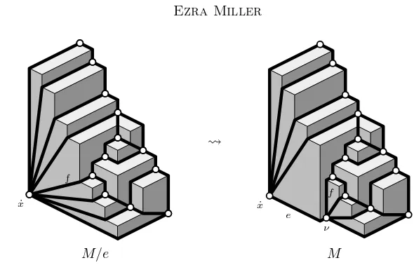
Proposition 4.1 LetM be a planar map with axial verticesx,˙ y,˙ z˙. Supposee
is the edge in the exterior cycle ofM leaving x˙ towardy˙, and thateborders no triangles inM∞( ˙x,y,˙ z˙). IfM/ecan be rigidly embedded in some grid surface, then so can M.
Proof. Letting ν ∈M be the other endpoint ofe, we haveν 6= ˙y because the unbounded region ofM∞containingeis not a triangle. The edge inM leaving
ν clockwise from e determines an edge f in any rigid embedding N ֒→ SV isomorphic to M/e. Note thatf ∈N does not contain the orthogonal rayYx˙
because f 6= e; and f 6⊃ Zx˙ because ν sits between ˙x and ˙y. Therefore the
orthogonal rayXω at the other endpointω off inN points toward ˙x. Assume all coordinates of vectors in V are even, by scaling. The claim is that the rigid geodesics in SV∪ν constitute a rigid embedding isomorphic to M, where the coordinates ofν are defined by
ν = (νx, νy, νz) = (|x| −˙ 1, ωy,0).
The addition ofν toV affects at most the rigid geodesics inN containing one of the following: an orthogonal rayXσ for some vertex σ∈ V pointing toward
˙
x; an orthogonal ray atν; orYx˙. All other rigid geodesics lie behind the plane x=|x| −˙ 1.
Ifσy< ωy, thenXσ is unaffected byν, while ifσy≥ωy, then ˙xandν are the only elements ofV precedingσ∨x˙ =σ∨ν+ (1,0,0). ThusXσpoints towardν if σy ≥ ωy, because ˙x 6¹ σ∨ν. The three orthogonal rays Xν, Zν, and Yν leaving ν point respectively toward ˙x, ω, and the vertex to which Yx˙ ⊂ SV points in N. Finally, Yx˙ ⊂ SV∪ν points toward ν. (Figure 3 illustrates the
transitionM/eÃM.) ✷
In the situation of Lemma 3.1, gluingM∩RintoM/Rmay involve contracting some of the tethers in (M/R)∪τ (M ∩R). For the rest of this section, let
M ֒→ SVM andN ֒→ SVN be rigid embeddings having respective axial vertices
˙
x,y,˙ z˙ and ¨x,y,¨ z¨, with τ ∈ M∞( ˙x,y,˙ z˙) a trivalent vertex having neighbors
α, β, γ. LetB be the region ofM ∪τN containingey¨andez¨.
Proposition 4.2 Assume that τ 6= ˙y, that Yx˙ points toward τ, and that no
f
˙ x
Ã
e f
ν ˙
x
M/e M
Figure 3: Uncontracting the lower-left edge
(if B has at least five vertices) both of e¨z and ey¨ in M ∪τ N yields a planar map possessing a geodesic grid surface embedding.
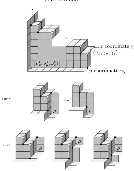
Proof. Paragraph headings are included below to make parts of the proof easier to follow and cross-reference.
Plan of proof
Given the conditions of the present proposition, assume all hypotheses and notation of Lemma 3.2, as well; this is possible by Lemma 2.1. If |VN| =n, scaleM so that all coordinates of vectors inVM are divisible byn+ 1. Until further notice (see the special construction for (8), below), assume in addition that the orthogonal rays Xτ, Yτ, Zτ all have length exactlym+ 1. Set
ν′ := τ+ν for ν ∈ VN.
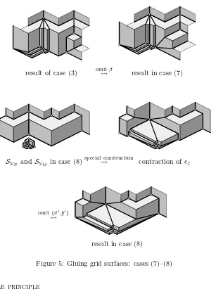
The plan of the proof is to split into a number of cases, each of which demands slightly different treatment. In every case, Lemma 2.1 allows a judicious choice of coordinates for vectors in VN. Most often, omitting one or more of the vertices {¨x′,y¨′,z¨′, β} from V leaves a set V such that the desired contraction of M ∪τN geodesically embeds into SV; two of the cases require additional fiddling with the surviving vertices to get the desired grid surface.
Eight cases
LetAandB be the bounded regions ofM∪τN containinge¨xandey¨,
vertices of A having u-coordinate Au. For instance, A(x) = {x}˙ ={α}, and
β ∈B(y).
Here is the list of constructions yielding SV. In each of (1)–(7), choose VN so that every coordinate of every vector in VN is at mostn; we treat the last case (8) separately later, since it involves somewhat different choices. Construct
V fromV = (VMrτ)∪(τ+VN) by omitting the indicated vectors, and (in (5) and (8)) making the specified alterations.
(1) To contract onlyex¨: omit ¨x′.
(2) To contractex¨ andey¨: omit ¨x′,y¨′.
To contractex¨ ande¨z...
(3) if no edge inN has endpoints{x,¨ z}¨ : omit ¨x′,z¨′. if{x,¨ z}¨ are the endpoints of an edge inN... (4) andAz> γz: omit ¨x′,z¨′.
(5) andAz=γz: omit ¨x′,z¨′; then add 1 toνzfor allν∈A(z)rγ. To contractex¨,ey¨, andez¨...
(6) if no edge inN has endpoints{y,¨ z}¨ : omit ¨y′ after (3)–(5). if{y,¨ z}¨ are the endpoints of an edge inN...
(7) andβx≥γx: omitβ after (3)–(5).
(8) andβx< γx: make the special construction below.
In general, observe that the only vertices connected to ¨x, ¨y, or ¨zinM∪τNare
α, β, γ, and some vertices inN. Also, one of (6)–(8) must occur ifBhas at least 5 vertices. Representative instances of the cases (1)–(8) appear in Figures 4 and 5.
Omitting vertices
In general, omitting one or more elements from V always leaves a set of pair-wise incomparable vectors. The vertex axiom will follow immediately in the applications below, in the sense that the surviving vertex vectorsV are in obvi-ous bijection with the vertices of the desired map. To check the rigid geodesic axiom after omitting one vertexν, we must verify that any orthogonal rayU
pointing towardνbefore the omission ofνpoints to some other uniquely deter-mined surviving vertex afterwards. This will show that the surviving vertices
V define a rigid embeddingL ֒→ SV for some mapL.
. ..
· · · · · ·
. .. .
. .
¨ x′
¨ y′
¨ z′
α
β γ
SV
omit ¨x′
à result in case (1)
omit ¨y′
à result in case (2)
SV in case (3) omit ¨x ′
à SVrx¨′
omit ¨z′
à SVr{x¨′,z¨′}
SV in case (4)
omit ¨x′
à SVrx¨′
omit ¨z′
à result in case (4)
SV in case (5)
omit{x¨′ ,¨z′
}
à SVr{x¨′,z¨′}
add
à result in case (5)
SV in case (6)
case (3)
à SVr{x¨′,z¨′}
omit ¨y′
à result in case (6)
result of case (3) omitÃβ result in case (7)
SVN andSVM in case (8)
special construction
à contraction of e¨z
omit{¨x′ ,y¨′
} Ã
result in case (8)
Figure 5: Gluing grid surfaces: cases (7)–(8)
Scale principle
We chose the relative sizes of VN and VM so that some arguments in what follows can rely on the following principle: Ifω, σ are two vectors whose coor-dinates are all divisible byn+ 1, thenω¹σif and only ifω¹σ+n1.
Rays leaving τ+VN
An orthogonal ray leaving ν′ ∈ τ +V
N and pointing toward ¨z′ in SV must be Zν′ ⊂ SV. We claim that after omitting ¨z′, the ray Z
ω∈ {ν′,z¨′, γ}. If ω ∈ τ +V
The rigid geodesics containing orthogonal rays Xν′ pointing toward ¨x′ before the omission and towardαafterwards account for all of the necessary edges in the contraction. It remains only to verify thatYα ⊂ SVrx¨′ points toward the
next vertex after ¨x′ whose z-coordinate is zero—that is, the counterclockwise next vertex after ¨x′ on the exterior cycle ofM ∪
τN. This easy argument is left to the reader, completing the proof of (1). Until the proof of (8), assume ¨
x′ has been omitted.
Proof of (2)
The orthogonal rays pointing toward ¨y′ in S
Vrx¨′ are Yν′ for some vertices ν ∈ VN, the ray Xβ, and possibly Yα (if ¨x and ¨y are the vertices of an edge in N). The arguments in ‘Rays in τ+VN’ and ‘Proof of (1)’ apply as well to the omission of ¨y′, including the fact that the ray X
β points toward the next vertex after ¨y′ whose z-coordinate is zero (which may be α). None of the edges incident to ¨y′ vanish (see ‘omitting vertices’), although X
β and the
Y-orthogonal ray at height z = 0 pointing toward ¨y′ point toward each other after omitting ¨y′, effectively contractinge
¨ y. Cases (3)–(5)
Every rigid geodesic incident to ¨z′inS
Vrx¨′ contains an orthogonal ray pointing
toward ¨z′, except the geodesic connecting αto ¨z′, if there is one (this occurs in (4) and (5) only, whereX¨z′ points toward αinSVrx¨′), and sometimes the geodesic connectingγ to ¨z′.
After omitting ¨z′, we will verify the rigid geodesic axiom at γ separately for each of (3)–(5), by checkingonlythat an orthogonal ray leavingγand pointing toward ¨z′ (if there is one) points instead to another surviving vertex after omitting ¨z′. Any other orthogonal ray in S
Proof of (3)
If Xγ points toward ¨z′ in SVr¨x′, and ν
′ is the vertex to which X
¨
z′ points in SVr¨x′, then Xγ points toward ν
′ ∈ τ +V
N after omitting ¨z′ by the scale principle (the hypothesis for (3) guarantees thatν′6= ¨x′). A similar statement holds by switching the roles ofxandy (but ν′ ∈τ+V
N is always guaranteed to exist, since ¨y′ has not been omitted). This verifies the rigid geodesic axiom atγ.
Proof of (4)
The assumptionAz> γzimpliesAy=γy, so thatXγpoints toward ¨z′inSVr¨x′.
Ifν ∈ Vrx˙ andνy< γy, thenνz> γz, by the region axiom. The omission of ¨
z′ therefore causes the rayX
γ ⊂ SVr{x¨′,z¨′}to point towardα.
Proof of (5)
The region axiom impliesγy < τy, soXγ does not point toward ¨z′. When Yγ points toward ¨z′, the rigid geodesic axiom holds forS
Vr{x¨′,z¨′} by the argument
in the proof of (3), although no elbow geodesic connectsαtoγin SVr{x¨′,z¨′}.
Now we verify that the addition procedure outputs a rigid geodesic embedding, and that an edge connecting α to γ is the only new rigid geodesic. We can safely ignore all orthogonal rays contained in rigid geodesics on the positive side of the planey=γy. All of the verticesω6∈Asatisfyingωy ≤γy must also satisfy ωz > γz by the rigid region axiom. The adding rule therefore causes
Xγ to point toward αafter omitting ¨z′. The orthogonal rays leaving vertices originally inA(z)rγ still point to the same vertices, by the scale principle. If
ω 6∈A(z)∪ {α}, then any orthogonal rayUω pointing towardν ∈A(z) before the addition still points toward the same vertexνafterwards, becauseωz> νz, whence the joinν∨ω remains unaffected. Finally, ifZα points toward a vertex in A(z) before the addition procedure, thenZαstill points to the same vertex afterwards, by the scale principle, whileYα remains unaffected.
Proof of (6)
No new phenomena occur here; see Proof of (3).
Technical lemma
The following result will be applied in the proofs of (7) and (8). For the proof of (8), note that it holds after any rescaling ofVM as in Lemma 2.1.
Let ω ∈ VM. If τx ≥ ωx ≥ βx, then ω ∈ {τ, β} or ωz ≥ γz. Similarly, ifτy ≥ωy≥αy = 0, thenω∈ {τ, α} orωz≥γz.
Proof of technical lemma. Supposeτx≥ωx≥βx, butωz< γz. Ifω6=τ, then
in VM. Thusβ ¹ω, so β =ω. Swap the roles ofxand y to prove the other statement.
Proof of (7)
First claim: The only orthogonal rays pointing toward β areYy¨′, and X ν for some vertices ν∈M. These verticesν all haveνz< m+ 1.
The final sentence of the first claim is easy, because otherwiseγ¹β∨ν. For the rest of the claim, use the inequalities Bx=τx> βx≥γx andBy =βy > τy ≥
γy, which follow from the hypotheses of (7). These implyγz =m+ 1 =Bz, thanks to the region axiom. By the technical lemma, any orthogonal ray Yν pointing towardβ inSV(and therefore inSVr{x¨′,z¨′}) must have eitherνx≥τx
or νz≥m+ 1. Whenνx≥τx, we getνy< βy and hence ¨y′ ¹ν∨β, soν= ¨y′. The case νz ≥m+ 1 is actually impossible, for it implies γ ¹ν∨β, so ν =γ is connected to β by an edge in M ∪τN; this cannot happen in (7) ifB has at least five vertices. The fact that βz = 0 rules out Zν pointing toward β, completing the proof of the first claim.
Now we verify that Xν ⊂ SVr{x¨′,β,z¨′} points toward ¨y
′ whenever X ν ⊂
SVr{x¨′,¨z′} points toward β. In other words, we need ω ¹ ν∨y¨
′ for ω ∈ V to imply ω ∈ {x¨′,z¨′,y¨′, β, ν}. If ω ∈ τ +V
N, then ωx = ¨y′x = τx implies
ω ∈ {y¨′,z¨′}. If ω ∈ V
M rτ, then either ωx ≤ βx, in which case ω ¹ β∨ν impliesω ∈ {β, ν}, orωz< m+ 1 in addition to τx ≥ωx≥βx, in which case
ω=β by the technical lemma.
It is easy to verify that ¨y′ points toward the next vertex after β having z -coordinate zero. Note that such a next vertex must exist, since the rigid geodesic leaving β and containing Zβ strictly decreases in x. This completes the proof of (7).
Special construction for (8)
The meet (componentwise minimum) of τ and γ is τ∧γ = (γx, γy,0) = γ− (0,0, m+ 1) sinceZτ points towardγin SVM. Observe that
ω∈ VM andτ∧γ¹ω implies ω∈ {τ, γ}. (9) Indeed, if τ6¹ω butτ∧γ¹ω, then eitherτx≥ωx≥γxor τy ≥ωy≥γy. The hypothesis γx > βx of (8) plus the technical lemma imply ωz ≥ γz, whence
γ¹ω.
It follows from (9) that the set
VM = (VM r{τ, γ})∪τ∧γ
τ so that τ−τ∧γ equals (1,0,0), (0,1,0), or (1,1,0), depending on whether
τy=γy,τx=γx, or neither.
Now chooseVN so that all of itsnonzeroxandy-coordinates lie in the interval [m−n, m], but all of its z-coordinates are no greater thann. Let
V = (VM rτ∧γ)∪(τ∧γ+VN),
and denote byνthe vectorτ∧γ+ν forν∈ VN. Our (final) goal is to show that the rigid geodesics inSV constitute an embedding of (M∪τN)/ez¨. After that, ex¨ and ey¨ can be contracted by omitting ¨xand ¨y, using the same arguments
appearing in Scale principle, Rays leavingτ+VN, Proof of (1), and Proof of (2).
Proof of (8)
Begin by mimicking as closely as possible the proof of Lemma 3.2. First,τ∧γ
is the unique vector in VM preceding τ∧γ+m1, by Lemma 3.2 applied to VM; this is why τ needs to be so close to τ∧γ. The vertex axiom for SV is immediate. Moreover, the part ofSVthat precedesτ∧γ+m1equalsτ∧γ+(the part of SVN preceding m1). Thus every vertex, rigid geodesic, or bounded
orthogonal ray in N ֒→ SVN gets translated by τ∧γ to the corresponding
feature inSV. Similarly, the parts ofSV andSVM not preceded byτ∧γagree, so any vertex, rigid geodesic, or bounded orthogonal ray inM ֒→ SVM survives in SV whenever it is contained in a (perhaps unbounded) region of M∞ not containingτ orγ, by the rigid region axiom.
The only orthogonal rays unaccounted for as yet for the rigid geodesic axiom areXx¨,Yy¨,Yα,Xβ,Z¨z, and any orthogonal rayUν ⊂ SV such thatUν⊂ SVM
points towardγandν6=τ. (Neither the rigid geodesic connectingτ toγinM
nor the orthogonal rays leaving γ in SVM play roles in this verification.) The
only case requiring significant effort are the Uν rays, which must point toward ¨
z inSV.
Suppose ω ¹ν∨z¨for some ω ∈ V. The technical lemma and (9) imply that
νz ≥γz for any τ 6= ν ∈ VM pointing toward γ, whence ν∨z¨= ν∨γ for any such ν. Therefore ω 6=ν implies ω ∈ τ∧γ+VN. On the other hand, either
νy < βy or νx < αx, because otherwiseβ or α precedesν∨γ =ν∨z¨. By the choice of scaling,ωy ≤νy < βy forcesωy ≤νy ≤βy−(n+ 3)< γy+m−n, whence ω = ¨z wheneverω ∈τ∧γ+VN. This argument also works with the roles ofxandy switched.
The above reasoning proves that the rigid geodesics inSV embedsome planar map L. To conclude that L ∼= (M ∪τ N)/ez¨, one last item remains: show
that no geodesics in M vanish. More precisely, whenever Xγ or Yγ does not point towardτinVM, we require it to point toward a vertex inVM that points back toward γ in SVM. Suppose Yγ ⊂ SVM does not point toward τ. Then γx < τx =Bx, whence γz =Bz by the region axiom, becauseγy < βy =By. If B(z) = {γ}, then Yγ ⊂ SVM must point toward β, because βx < γx. This
argument works for Xγ, but the reason why Xγ cannot point toward α is different: it is ruled out by the statement of the Proposition. ✷
Recall the conventions set before the statement of Proposition 4.2.
Proposition 4.3 Supposeτ = ˙xis trivalent. Contracting neither, either, or (if B has at least five vertices) both of e¨z and ey¨ in M ∪τ N yields a planar map possessing a rigid embedding.
Proof. Pretend ex¨ has already been contracted, and apply the constructions
in the proofs of (6)–(8) in Proposition 4.2. (In reality, only (6) and (7) are required here, given the symmetry switching the roles of yandz). ✷
5 Triconnectivity and rigid embedding
Theorem 5.1 (Rigid embedding) A planar mapM with given axial vertices ˙
x,y,˙ z˙ can be rigidly embedded in a grid surface if and only if the extended map
M∞( ˙x,y,˙ z˙) is triconnected. In particular, every triconnected planar map can be rigidly embedded.
Proof. (⇒) Let M ֒→ SV be an axial rigid embedding, and delete two ver-tices ν, ω from M∞. If {ν, ω} ⊂ {x,˙ y,˙ z}˙ then each remaining vertex has an orthogonal flow to the third axial vertex, by independence of the orthogonal flows to ˙x,y,˙ z˙. If {ν, ω} 6⊂ {x,˙ y,˙ z}˙ then what remains of the exterior cycle is connected, and every vertex in the deletion still has an orthogonal flow to the exterior cycle.
(⇐) Induct on the sum of the number of regions and the number of edges inM, observing that the minimal sum of five is attained only whenM is a triangle. Assume the notation of Section 3, and supposeM is not a triangle. Lettinge
be the edge leaving ˙xtowards ˙y on the exterior cycle ofM, we claim that at least one of the following occurs:
1. The endpoints ofeare ˙xand ˙y.
2. The edgeedoes not border a triangle inM∞( ˙x,y,˙ z˙), andM/eis tricon-nected.
3. The edgeedoes not contain ˙y, andM contains a proper ringCfor which ¨
x=∞.
4. The edgeedoes not contain ˙y, andM contains a proper ringCfor which (a) ¨x= ¨x= ˙x;
(b) ¨y is the other endpoint ofe, and ¨y6= ˙y(that is, ¨y6=∞); and (c) ¨z does not lie between ˙xand ˙z on the exterior cycle ofM, and no
Proposition 1.1.2. Note that C is proper because ¨y6= ˙y. LetC be a maximal such ring.
The first half of 4(c) holds; if not, construct a ring satisfying option 3 as follows: replace the arc ofCconnecting ˙xto ¨zwith the arc traversing the exterior cycle from ˙xto ¨zand thenez¨(the latter only if ¨z6= ¨z). The second half of 4(c) also
holds, for if an edge f outsideC connects ˙x to ¨z, then replace the arc of C
connecting ˙xto ¨z in C byf and ez¨(if ¨z6= ¨z). The resulting cycle is a larger
ring satisfying the condition defining C, contradicting maximality. Finally, 4(a) holds by the failure of option 3: Cdoes not contain the edge ofM leaving
˙
xtoward ˙zon the exterior cycle ofM.
Given the first option, M has a proper ring C, with ¨z = ¨z = ˙z, containing every bounded region of M except the one containing e. Let M ∩R ֒→ SV be a geodesic embedding, whereRis the union of regions contained withinC. Leaving ˙x,y˙fixed while adding 1 to thez-coordinates of every other vector inV
yields a grid surfaceSV′ whose rigid geodesics constitute an embedding ofM; the easy proof is omitted.
Given the second option, use Proposition 4.1. Given the third or fourth option, use Lemma 3.1 withM =M/Rand N =M ∩R, along with Proposition 4.3 for option 3, or Lemma 3.2 and Proposition 4.2 for option 4. The ‘five vertex’ conditions in Propositions 4.2 and 4.3 are always satisfied when reconstruct-ingM from the tethered gluing (M/R)∪τ(M ∩R), becauseM is simple and
triconnected. ✷
The next corollary clarifies the close connection between grid surfaces and order dimension for posets. It shows that Theorem 5.1 generalizes the three-variable special case of [BPS98, Theorem 6.4], which is presented in the equivalent language of monomial ideals.
Corollary 5.2 (Brightwell–Trotter [BT93])The vertices, edges, and bounded regions of any triconnected planar map form a partially ordered set of order dimension≤3.
Proof. Theorem 5.1 and Corollary 2.5. ✷
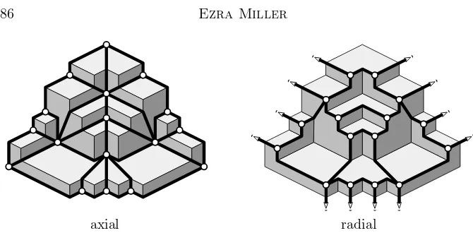
Example 5.3 Theorem 5.1 is stronger than Corollary 5.2, even for triconneted maps. In general, every inclusion of the vertex-edge poset ofM into N3yields an inclusion of the vertex set V ֒→ SV such that each edge of M is a rigid geodesic inSV. What fails is that there may be orthogonal rays inSVthat are not contained in any edges ofM. Faces such as the central face in Figure 6 are
then forced to lie off ofSV. ✷
Remark 5.4 Rigid embeddings give a fresh perspective on a standard fact, known as Menger’s theorem: IfGis a triconnected planar graph andν, ω∈G
֒→
Figure 6: A vertex-edge-face poset embedding that is not a geodesic embedding
a new map M′ by drawing a small circle C around ν and adding new ver-tices ν1, . . . , νr wheree1, . . . , er intersectC. Then set Mν = del(M′;ν), with underlying graphGν. ClearlyGν is triconnected.
Choose a plane drawing ofGν in whichCis the exterior cycle, and letGν ֒→ S be an axial geodesic embedding compatible with some (any) choice of axial vertices ˙x,y,˙ z˙∈C. The orthogonal flows fromωto ˙x,y,˙ z˙ inGν first intersect
C at points νix, νiy, νiz, giving rise to truncated orthogonal flows [ω, νiu] for u∈ {x, y, z}. Connecting [ω, νiu] toνvia the arc inGbetweenνiu andνyields
independent paths inGfromω toν.
Part II
Monomial ideals 6 Betti numbers
Letk be a field, and consider the polynomial ringR =k[x, y, z] with theZ3 -grading in which deg(x) = (1,0,0), deg(y) = (0,1,0), and deg(z) = (0,0,1). Use IV = hmν | ν ∈ Vi to denote the ideal generated the monomials
mν =xνxyνyzνz forν ∈ V. The integer points inhVicoincide with the
expo-nent vectors on monomials in IV, and V is axial if and only ifIV is artinian, containing a power of each variable.
Any principal monomial ideal hmi is a free Z3-graded R-module of rank 1. If φisZ3-graded homomorphism Lhmqi ←−Lhmpiof degree zero, then we can express φ as a monomial matrix. This is a matrix whose entries λpq ∈k are scalars, and whose pth row (resp.qth column) is labeled by the monomial mp (resp. mq) that generates the corresponding pth source (resp. qth target) summand. Of course,λpq= 0 whenevermq does not dividemp, because then there are no nonzero Z3-graded maps hm
qi ← hmpi. The map φ is called minimal if alsoλpq = 0 whenevermp =mq. See [Mil00a, Section 2] for more on monomial matrices.
We considerfree resolutionsofIV that are exact sequences having the form
F.: 0←IV φ0 ←− F0
φ1 ←− F1
φ2
←− F2←0, (10)
minimal ifφ1andφ2are minimal (for any such direct sum decomposition). The
Betti numberβi,α(IV) is the number ofmip equal tomα, whenF.is minimal. This homological data reflects the local properties ofSV near the vectorαvia theKoszul simplicial complexofV at α∈N3,
Kα(V) = {σ∈ {0,1}3|α−σ∈ hVi}, which is a subcomplex of the abstract triangle ({0,1}3,¹).
Proposition 6.1 ([Hoc77, Roz70]) βi,α(IV) = dimkHei−1(Kα(V);k)is the dimension of the(i−1)st reduced simplicial homology ofK
α(V)with coefficients in k.
The small number of simplicial complexes on three vertices seriously limits the possibilities for nonzero Betti numbers.
Lemma 6.2 If V ⊂N3 and i∈N then βi,α(IV)6= 0 for at most one α∈Z3. If βi,α is nonzero then βi,α= 1 unless Kα(V) has 3 vertices and no edges (so
β1,α= 2).
Proof. Use the previous proposition, and list all simplicial complexes on 3
vertices. ✷
7 Cellular resolutions
SupposeM is a cell complex (precisely, a finite CW complex) of dimension 2 whose cells P have vector labels αP ∈ N3, in such a way that αP ¹ αP′ if
P lies in the closure of P′. For instance, if the vertices have natural labels, then defineαP to be the join of the labels on the vertices ofP. Such alabeled cell complex determines monomial matrices φvertex, φedge, and φregion for a
cellular free complexFM, by labeling the rows and columns of matrices for the boundary map of the ordinary chain complex of M with the monomialsmαP.
UsingP also to denote the basis vector of a rank 1 freeR-modulehmαPi, the
cellular free complex FM takes the form
φvertex φedge φregion
0←IV ←−−−−
M
verticesν
R·ν ←−− M edgese
R·e ←−−−− M regionsF
R·F ←0.
(11) We say M supports FM; see [BS98, Mil00a] for more on cellular monomial matrices.
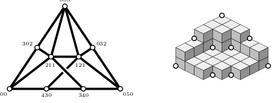
Example 7.1 Let IV = hx, y, zi2 = hx2, y2, z2, xy, xz, yzi. The orthogonal raysXyz, Yxz, Zxymeet at a single point not inV, so there can be no planar map geodesically embedded in SV. However, hx, y, zi2 still has a minimal cellular
resolution: connect the midpoints of the edges of a triangle, and delete any one of the three interior edges. Label the resulting planar map M with x2, y2, z2
on the corners of the outside triangle; xy betweenx2 and y2; yz between y2
and z2; andxz betweenx2 and z2. Label the edges and regions of M by the
joins of their vertex labels. ✷
Although the mapM in the above example fails to embed geodesically inSV, the extended map M∞(x2, y2, z2) is still triconnected. This phenomenon is
general. In the following proposition, we do not require planarity ofM, so we useG∞( ˙x,y,˙ z˙) to mean the abstract graph obtained fromGby adding a new vertex∞connected to each of ˙x,y,˙ z˙.
Proposition 7.2 If the labeled cell complex M supports a minimal free reso-lution of an artinian ideal IV, and the1-skeleton of M is a graphG, then the extended graphG∞( ˙x,y,˙ z˙)is triconnected, wherex,˙ y,˙ z˙ are the vertices whose labels lie on the axes.
Proof. Givenν ∈ V with ν 6= ˙z, the orthogonal ray Zν leavingν has its head at some vector α ∈ N3 for which Kα(V) is disconnected; indeed, the vertex (0,0,1) is isolated in Kα(V). Choose a vertex ω′ 6= ν preceding α, so that
mα−νν−mα−ω′
ω′ ∈ ker(φ
vertex). Sinceα−ν = Z(ν) lies on the z-axis Z,
there must be an edge e ∈ M connectingν to a vertex ω (possibly different fromω′) such thatφ
edge(e) =zdν−mν∨ω−ωωfor somed∈N. Clearlyωx¹νx andωy¹νy.
Repeating the procedure withω in place ofν, and withxory in place ofz, we find thatM contains paths analogous to orthogonal flows fromν to each axial vertex ˙x,y,˙ z˙. As in Section 2, these paths are independent, intersecting only
atν. ✷
8 Graphs to minimal resolutions
Lemma 8.1 If M ֒→ SV is a geodesic embedding, then β1,α(IV) 6= 0 if and only if α =ν∨ω for some elbow geodesic [ν, ω] ∈ M, and β1,ν∨ω(IV) = 1 in this case.
Proof. Assumeβ1,α(IV)6= 0. ThenKα(V) is disconnected by Proposition 6.1, and this occurs if and only if Kα(V) contains an isolated vertex. An isolated vertex ofKα(V) occurs if and only ifαlies on an orthogonal ray leaving some vertex ν ∈ V. Therefore, α=ν∨ω for someω 6=ν by the edge axiom. Since [ν, ω] is an elbow geodesic,Kν∨ω(V) cannot have three isolated points because three orthogonal rays cannot meet at the point ν∨ω in the relative interior of
Here is a result that sometimes reduces statements about arbitrary geodesic or rigid embeddings to axial ones. Its straightforward proof is omitted.
Lemma 8.2 Append axial vertices toV by letting V =V ∪ {u˙ | SV∩U =∅} for sufficiently large |u|˙ . A planar map M is geodesically embedded in SV if and only if N = del(M;VrV) is geodesically embedded inSV. Furthermore,
M ֒→ SV is rigidly embedded if and only ifN ֒→ SV is rigidly embedded.
Lemma 8.3 LetM ֒→ SV be a geodesic embedding, andSVmax the set of points in SV maximal under the partial order induced by the relation¹onR3. Then
α∈ Smax
V ⇔β2,α(IV)6= 0⇔ α=αF is the join of the vertices in a bounded region F ofM.
Proof. For the equivalenceα∈ Smax
V ⇔β2,α(IV)6= 0, use the fact thatKα(V) is the boundary of the triangle; the easy details are omitted. The equivalence
α ∈ Smax
V ⇔ α = αF holds for all vertex sets V if it holds when V is axial. Indeed, using the notation and result of Lemma 8.2, the maximal points of
SV are still maximal inSV, while the points inSVmaxrSVmax are exactly those havingu-coordinate|u|˙ for someusuch thatSV∩U =∅, by the region axiom applied to SV. The bounded regions of N having such joins disappear upon deleting ˙u.
Assume henceforth that M ֒→ SV is axial. If ρ ∈ SV has some coordinate
ρu = 0, then ρ6∈ SVmax because adding ε to any other coordinate ofρ yields another point in SV. Therefore each maximal point of SV lies in a bounded region of M. When F is such a bounded region, the region axiom implies
αF ∈ SVmax, because some vertexν∈ V strongly precedesαF+εu˙ for anyε >0 andu∈ {x, y, z}.
Every pointρ on a given elbow geodesic [ν, ω] precedes ν∨ω by definition, so
ρ¹ν∨ω¹αF whenever [ν, ω] ⊆ F. Any point σ on the line segment in R3 connectingρto αF therefore satisfiesρ¹σ¹αF, whenceσ∈ SV. It follows thatF is the union of such line segments, so every point ofF precedesαF. ✷ Theorem 8.4 Given a geodesic embeddingM ֒→ SV, the cellular free complex
FM is a minimal free resolution ofIV.
Proof. Sinceβi,α(IV)6= 0 if and only ifβi,α(IV) = 1 by Lemmas 6.2 and 8.1, it makes sense simply to speak of the ith Betti degreesα, for whichβ
i,α= 1. The zeroth, first, and second Betti degrees are the labels on the vertices, edges, and regions of M, respectively, by Lemmas 6.2, 8.1, and 8.3. Any minimal free resolution F.of IV as in (10) therefore takes the form of (11), at least as a homologically graded module; that is,F.∼=FM abstractly as modules. We need to show that some choice of this abstract isomorphism is a homomorphism ofcomplexes.
Identifying the homological degree zero parts ofF.andFM, the zeroth homol-ogy of FM surjects ontoIV because the image of φedge is clearly contained in
exists a homomorphismψ:FM → F.lifting the surjection on zeroth homology and the isomorphism in homological degree zero.
Supposee∈ FM maps to ψ(e) =Pmje′j, where eachmj ∈R is a monomial with nonzero scalar coefficient, and eache′
j denotes the generator ofF1
corre-sponding to the edgeej ∈M. The elbow geodesice= [ν, ω] inM contains an orthogonal ray Uν, so that ±φ1(Pmje′j) = mν∨ω−νν−mν∨ω−ωω, where the first term is mν∨ω−νν =mU(ν)ν. ThusmU(ν)ν=u|Uν|ν appears with nonzero
scalar coefficient in φ1(mje′j) for some j. Since there is a unique first Betti degree α satisfying α−ν ∈ U, namely αe = ν∨ω, it must be that e′j = e′ and mj is a nonzero scalar. Nakayama’s lemma implies ψ1 : (FM)1 → F1 is
surjective, and hence an isomorphism by rank considerations.
No summandR·F ⊂ FM can map to zero inF2 becauseφregion(F) is nonzero
in FM, andψis an isomorphism in homological degree 1. On the other hand, the second Betti degrees are pairwise incomparable by Lemma 8.3. Thusψ(F) is some nonzero scalar multiple of the unique generator of F2 in degree αF. The map ψ is therefore an isomorphism in homological degree 2, completing
the proof. ✷
Corollary 8.5 A planar mapM with axial vertices x,˙ y,˙ z˙ supports a mini-mal free resolution of an artinian monomial ideal if and only if M∞( ˙x,y,˙ z˙)is triconnected. In particular, every triconnected planar map supports a minimal free resolution.
Proof. ‘Only if’ is Proposition 7.2; apply Theorem 8.4 to Theorem 5.1 for ‘if’.
✷
9 Uniqueness vs. nonplanarity
Continuing with the analogy at the beginning of the Introduction, circle pack-ings and polytopes that realize planar graphs are unique up to M¨obius transfor-mation and spherical rotation, respectively (see [Zie95] for discussion and ref-erences). Rigid embeddings M ֒→ SV for a fixed planar map are similarly not unique: at the very least, any order-preserving bijection ofV as in Lemma 2.1 gives another rigid embedding. Of course, such bijections affect neither the combinatorics nor the algebra. In fact, rigid embeddings are uniquely deter-mined by the algebraic properties of the grid surface in question, specifically the minimal free resolution of the corresponding monomial ideal.
Corollary 9.1 When M ֒→ SV is rigidly embedded, M is the unique cell complex supporting a minimal cellular free resolution ofIV.
500 050 005
211 121
302 032
430 340
Figure 7: Nonplanar minimal free resolution
whose degrees precedeαF. The only such cycle consists of all the edges whose degrees precedeαF, by the rigid region axiom forF′ inM (by Lemma 8.2 the rigid region axiom holds for nonaxial grid surfaces). ✷
Nonrigid monomial ideals can have many distinct isomorphism classes of min-imal cellular resolutions; [MS99, Figure 4] depicts an example of this phe-nomenon. In fact, the bad behavior gets much worse.
Example 9.2 Minimal cellular resolutions of ideals in k[x, y, z] need not be supported planar cell complexes. In fact, explicit examples crop up with even the smallest violations of rigidity. For instance, let
V = {(4,3,0),(3,4,0),(3,0,2), (2,1,1),(1,2,1),(0,3,2)}
and V = V ∪ {(5,0,0),(0,5,0),(0,0,3)}. The cell complex M depicted in Figure 7 consists of five triangles in addition to the three quadrilaterals with vertices
{500,430,121,211}, {430,121,211,341}, {050,121,211,340}.
Label the edges and regions by the joins of their vertex labels. ThatM supports a minimal free resolution ofIVcan be checked by verifying for eachα¹(5,5,3) that M¹α is acyclic [BS98, Corollary 1.3]. ThatM cannot be planar follows by contracting the edges labeled 530 and 350 while deleting the edges labeled 312 and 132 to get the complete graphK5 as a minor of the 1-skeleton. ✷
10 Deformation and genericity
Given a finite subsetW ⊂R3, write∨W for the join of the vectors inW, and
set mW=m∨W. Following [BPS98], define theScarf complexofV, ∆V = {W ⊆ V | if∨W′=∨W for someW′ ⊆ V thenW′=W},
with a natural label∨W, and the resulting cellular free complexF∆V is called the free Scarf complex of IV. The Scarf complex is planar by virtue of its containment in thehull complex[BS98], so the union of its edges and vertices is a planar map. This planar map has already appeared, in Section 2: two verticesν, ω∈ V are connected by a rigid geodesic if and only if{ν, ω} ∈∆V. Under special circumstances, the Scarf complex is rigidly embedded inSV. To be precise, call V strongly generic if no two distinct elements of V share a nonzero coordinate. In other words,νu=ωu6= 0 for someu∈ {x, y, z}implies
ν =ω.
Corollary 10.1 (Bayer–Peeva–Sturmfels [BPS98, §3]) The free Scarf complex F∆V minimally resolvesIV when V is strongly generic.
Proof. Strong genericity easily implies that every orthogonal ray is contained in a rigid geodesic, so the Scarf graph rigidly embeds in SV. It is straight-forward to verify that the labels on triangles (2-dimensional faces) in ∆V are maximal inSV. Furthermore, every maximal point ofSVhas exactly three vec-tors inV preceding it by Lemma 8.3, the region axiom, and strong genericity. Therefore, all maximal points are labels on regions in ∆V, and the result holds
by Theorem 8.4. ✷
Since the definition of the Scarf complex depends only on the coordinatewise order of the exponents of the generators, it also makes sense for (formal) mono-mials with real exponents inRn. This makes way for the following definition. LetQdenote the rational numbers. AdeformationǫofVis a choice of vectors
ǫν = (ǫν
x, ǫνy, ǫνz)∈Q3 for eachν ∈ V satisfying
νu< ωu ⇒ νu+ǫνu< ωu+ǫωu, and νu= 0 ⇒ ǫνu= 0 foru∈ {x, y, z}. In practice, everything we do is invariant under scaling ofV, so we will always assumeVǫ={ν+ǫν |ν∈ V}consists of integer vectors. Set
νǫ=ν+ǫν.
The sole purpose of theǫvectors is to break ties one way or the other between equal nonzero coordinates of vectors inV. In this manner, deformations of V
are closer to being generic thanVis. The verbspecializeis used here to indicate that a deformation (generization) is being reversed; thusV is aspecialization ofVǫif the latter is a deformation of the former.
One particular deformation will play a key role in the coming sections. To define it, letV(u, a) ={ν ∈ V |νu=a} for each 0< a∈Nand u∈ {x, y, z}. Up to order-preserving bijection (as in Lemma 2.1), there is a unique deformation ǫ
satisfying the following condition as well as its analogues via cyclic permutation ofx, y, z: