COMBINATORIAL CLUSTERING AND ITS APPLICATION TO 3D POLYGONAL
TRAFFIC SIGN RECONSTRUCTION FROM MULTIPLE IMAGES
B. Valleta,∗, B. Soheiliana, M. Brédifa
a Université Paris-Est, IGN/SRSIG, MATIS, 73 avenue de Paris, 94165 Saint-Mandé, FRANCE (bruno.vallet, bahman.soheilian, mathieu bredif)@ign.fr
recherche.ign.fr/labos/matis/∼(vallet, soheilian)
WG III
KEY WORDS:3D reconstruction, mobile mapping, urban areas, clustering
ABSTRACT:
The 3D reconstruction of similar 3D objects detected in 2D faces a major issue when it comes to grouping the 2D detections into clusters to be used to reconstruct the individual 3D objects. Simple clustering heuristics fail as soon as similar objects are close. This paper formulates a framework to use the geometric quality of the reconstruction as a hint to do a proper clustering. We present a methodology to solve the resulting combinatorial optimization problem with some simplifications and approximations in order to make it tractable. The proposed method is applied to the reconstruction of 3D traffic signs from their 2D detections to demonstrate its capacity to solve ambiguities.
1. INTRODUCTION
Traffic signs are important road features that provide nav-igation rules and warnings to drivers. Their detection and identification in image is largely investigated by the ADAS (Advanced Driver Assistance System) research community since the 90s. Many different pattern recognition techniques are applied for this purpose. A recent state-of-the art in this field can be found in the paper presented by (Fu and Huang, 2010). Most of the traffic sign extraction systems deal with detection and classification of signs in single images. Some systems integrate the detection and classification in a track-ing mode (Fang et al., 2003, Lafuente-Arroyo et al., 2007, Meuter et al., 2008). Consequently, more reliable decisions can be made using multi-frame rather than single-frame in-formation. Overall, there is a large amount of research work on detection and classification of traffic signs using single or multi-frame image data. In contrast, fewer authors investi-gated 3D reconstruction and localization of traffic signs, al-though, it is required for several applications:
• Road inventory and update,
• Visibility analysis in urban areas,
• Virtual reality and 3D city modeling,
• Vision based positioning using visual landmarks.
1.1 Previous works
The problem of 3D traffic sign reconstruction from multiple images acquired by a Mobile Mapping System (MMS) was first investigated by (Timofte et al., 2009). Plausible corre-spondence between 2D detections of traffic signs on different
∗Corresponding author.
images are computed based on geometric and visual consis-tency criteria. A 3D traffic sign hypothesis is then generated for each consistent pair of signs. Finally, a Minimum De-scription Length (MDL) approach is used to select an opti-mal subset of 3D traffic sign hypotheses. The method reaches 95%of correct reconstruction rate with an average localiza-tion accuracy of 24cm, which can deteriorate to1.5min some cases.
An inventory system based on stereo vision and tracking was also developed for traffic sign 3D localization (Wang et al., 2010). Pairs of corresponding 2D detections of traffic signs are deducted from tracking them in successive images. Two stereo-based approaches called single-camera (stereo from motion) and dual-camera (rigid stereo base) are studied. Traf-fic sign localization accuracy varies from1−3mfor single-camera to5−18mfor dual-camera.
paper is to propose a generic framework to handle such am-biguities. The scope thus goes way beyond the application to traffic sign as our methodology can be applied more gen-erally to disambiguate the 3D reconstruction of similar ob-jects (motion capture trackers, crowds, animal swarms, par-ticle clouds...) from 2D detections.
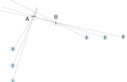
Figure 1: Clustering ambiguity: Two 3D signs (A, B) and six 2D detections (1-6). The correct clustering is (1,2,3) (4,5,6) but a greedy approach will usually give (1,2,3,5,6) (4) leading to a poor reconstruction of sign A and an omission of sign B that cannot be reconstructed from a single image.
1.2 Positioning
In the aforementioned 3D reconstruction approaches, this clus-tering problem is handled differently:
• The MDL approach of (Timofte et al., 2009) is lim-ited to pairwise matchings, in which case a global op-timum can be obtained by Integer Quadratic Program-ming (Leonardis et al., 1995). Conversely, we are trying to exploit as many views as possible in order to increase the accuracy of 3D reconstruction.
• (Wang et al., 2010) track the detections in image se-quences. If the same sign is seen by different cameras of the mobile mapping system or if the tracking fails (because of occlusions for instance) it might be recon-structed multiple times.
• (Soheilian et al., 2013) iteratively groups the 2D detec-tions in a greedy manner then ensures unicity of attri-bution (a 2D detection cannot be used to reconstruct more than one 3D sign). This heuristic does not ensure global optimality as (Timofte et al., 2009) does, but al-lows grouping more than 2 signs which helps enhancing the precision of the 3D reconstruction.
The aim of this paper is thus to propose a generic approach in a well justified theoretical framework to solve this clustering problem by exploiting the geometric consistency though a dissimilarity metric. Section 2. poses this clustering problem and proposes a method to solve it. Section 3. presents the application of our combinatorial clustering to the problem of 3D reconstruction of similar objects from their detections then specifies it to polygonal traffic signs. Finally we will conclude and open perspectives in Section 4.
2. COMBINATORIAL CLUSTERING
Combinatorial clustering is the generic tool that we introduce to solve the problem of reconstructing similar objects. The major lock is that it is very hard to know if two 2D detections correspond to the same 3D object, so we need a measure on the compatibility of 2D detections that is not a simple aggre-gation of a pairwise measures.
2.1 Problem formalization
In this section, we will call:
• Nn={1, ..., n}the firstnpositive integers
• O ={oi}i∈Nn: thenobjectsoithat we wish to clus-ter. For traffic signs, objects are the 2D detections and clusters corresponds to the 2D signs used to reconstruct a single 3D sign.
• P art(O)the set of parts ofO: P art(O) ={S|S ⊂ O}
• P(O)the set of partitions ofO:
P(O) = {{S1, ..., Sm}|Si ∈ P art(O)/∅andSi∪
Sj=∅andSSj=O}
• |S|the number of elements in the setS(cardinal).
LetD :P art(O)→R+be a measure of the dissimilarity
of a subset of objects.Dshould satisfy:
1. ∀i∈ Nn, D({oi}) = 0: Singletons (individual
ob-jects) are not dissimilar.
2. S1∩S2=∅ ⇒D(S1∪S2)≥D(S2) +D(S2): the
dissimilarity of a set is larger that the dissimilarity of any of its partition (or at best equal).
These two conditions imply thatDincreases when adding a new object to a set:
D(S∪ {oi})≥D(S) +D({oi}) =D(S) Most measures typically used for clustering satisfy these two conditions.Dimplies naturally a measure overP(O):
D({S1, ..., Sm}) = X
j
D(Sj)
Making no assumptions on the number of clusters, cluster-ing should find the partition that minimisesDover P(O). To avoid the trivial solution of making only singletons (in which case the total dissimilarity is 0), we should however also minimize the number of clusters in the partition, such that we pose the problem of combinatorial clustering as find-ing:
argminP∈P(O)E(P) =|P|+D(P) (1)
We will refer toEas the energy to be minimized.Dshould be chosen or scaled such that merging two subsetsS1andS2
S2)< D(S1) +D(S2) + 1) because in this case the energy
For 3D traffic signs reconstruction,Dcan be the residuals of a reconstruction of a sign from the 2D detections normalized by an estimate of the uncertainty on the image orientations (cf Section 3.2).
The problem posed above is very generic and can be applied to a broad variety of problems:
• Points clustering: the objects are points inRnand the
dissimilarity is the variance of a subset of these input points.
• Unsupervised classification: same as above with a vec-tor of features.
• Shape detection (such as RANSAC, Hough): the ob-jects are points inRnand the dissimilarity is the sum of residuals of a least square estimate of a subset of point by the shape to detect.
• Reconstruction of similar 3D shapes: objects are 2D de-tections of the similar 3D shapes and the dissimilarity is a normalized sum of residuals of the 3D reconstruction of an object from a subset of detections (cf Sections 3.1 and 3.2).
We will now propose a methodology to solve this combinato-rial clustering problem, that is to find a minimum (or at least a good approximation) of (1) over all possible partitions of the set(O)of input objects to cluster. To our knowledge, the numerous clustering methods that have been developed in the fields of computer vision and machine learning mainly deal with bivariate similarity measures (the dissimilarity measure is only defined for a pair of object), such that the dissim-ilarity of a set is sum of the pairwise dissimilarities of its constituents. For our specific problem, such approaches are insufficient as a very high similarity can be coincidental for detection corresponding to different 3D objects. This is why we investigated means to solve this more general clustering problem.
2.2 Compatibility graph
The number of partitions of a set ofnelements is the Bell number|P(O)| = Bnthat increases (very roughly) asnn which is even faster than exponential. Minimizing (1) over all possible partitions of the set(O)thus cannot be done by brute force in reasonable time for more than 20 objects (for whichB20≈5.1013) while we were regularly confronted to
problems of size exceeding 100 in the context of road sign reconstruction. In this paper, we propose heuristics to make this problem tractable for large number of objects.
The first simplification of this problem is to list pairs of in-compatible objects and forbid putting them in the same set.
In other terms, we propose to find a criterion ensuring that two objectso1ando2are not in the same part of the optimal
solution. We found that the criterionD({o1, o2})>2gives
such an insurance, because in this case:
E({o1, o2, o3, ..., om}) = 1 +D({o1, o2, o3, ..., om})≥
1+D({o1, o2})+D({o3, ..., om})>3+D({o3, ..., om}) =
E({o1},{o2},{o3, ..., om})
This result has a simple geometric interpretation: the mini-mization ensures that the clusters have a maximum radius of 1 (in normalized dissimilarity), so two objects further than 2 cannot belong to the same cluster.
If more is known onD, a finer incompatibility criterion should be investigated (cf Section 3.2 in the case of 3D traffic signs reconstruction). This incompatibility relationship allows us to build an object compatibility graphGC where nodes are objects and an edge exists between two nodes if the corre-sponding objects are compatible (cf Figure 2, last page). Ac-ceptable partitions will then be partitions of this graph into cliques (subsets of the graph where each node is connected to each other, or equivalently sets of objects all compatible one with another). This approximation decreases drastically the number of possible partitions, especially if the compatibility criterion is well chosen. It also naturally splits the problem into smaller problems given by the connected components of GCthat can be processed separately (in different threads and on different machines).
Finding the optimal partitions of a connected componentC of a graph in cliques can be done in the following way:
1. List all the cliquesCkofCand compute their energies
E(Ck).
2. Build a clique compatibility graphCCwhere the nodes are the enumerated cliquesCk, and there is an edge iff cliques are non intersecting (intersecting would mean the same object belongs to two clusters).
3. Find the maximal clique of minimum energy inC. A maximal clique ofCcorresponds to a partition ofCin non overlapping cliques. The standard being maximum weighted clique, we will simply take the opposites of the individual clique energies.
Note that we handle two different types of cliques:
1. Cliques ofCthat are sets of objects compatible one with another (potential clusters).
2. Maximal cliques ofCC that define partitions ofC in cliques (of the previous type).
2.3 Clique enumeration
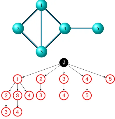
1
Figure 3: A simple graph (top) and its clique tree (bottom). Each red nodetkcorresponds to the clique of the graph de-fined by listing the nodesnifrom∅totk
1. Create the tree roott0labelled with∅ = C0 and add
one child to this root labelled withnifor each nodeni ofG.
2. For each tree nodetk, labelled withnilist all the nodes
nj(j > i)ofCthat are connected to all nodes inCkand add a child totklabelled withnjfor each of them. The criterion(j > i)ensures that each clique is enumerated only once (with nodes in increasing order).
3. Iterate step 2 recursively on the new tree nodes until no new node is found.
The energyE(Ck)can be computed efficiently and stored on each tree node during this construction, especially if the update of the dissimilarity measureD(Ck)is a simple up-date of the dissimilarity of a sub-clique ofCk(given by the father node oftk). For large, highly connected graphs, this construction may exceed the memory size of the machine. In our experiments, this happens for connected components with more than 200 nodes and 3000 edges. We propose a solution to that problem in Section 2.5.4.
2.4 Maximum weighted clique
The maximum weighted clique problem is rather classical and efficient implementations exist to solve it, such as Cli-quer (Niskanen and Östergård, 2003). However, the num-ber of enumerated cliques grows rapidly with the numnum-ber of nodes and edges ofC, which makes the maximal clique problem too long to run. We can however give a certain time budget to the algorithm and ask it to give the best so-lution found after this amount of time if the optimal soso-lution cannot be found. In this case, we will compare the solu-tion with a greedy search (iteratively add the best clique not overlapping previously added cliques) and take the best. In extreme cases (more than105enumerated cliques) even the
graph construction may exceed memory size so we directly choose the greedy solution.
2.5 Improvements
For clarity, we have only given the core of the method in the previous sections. In our implementation, we have added several useful improvements to enhance the quality of the re-sult in the cases where optimality cannot be guaranteed and reduce the computing time and memory footprint of the al-gorithm.
2.5.1 Singletons removal By definition, singletons have an energy of 1 because their disparity is null. As singletons are cliques, they should be added to the clique compatibil-ity graph CC, which increases its size by n. However, a simple modification of the energy allows to bring their en-ergy to 0 making singletons indifferent (they can be added or not to the solution without modification to the energy):
E(S) = 1 +D(S) +|S|BecauseP|S|over a partition is exactly the numbernof objects, this only corresponds to adding the constantnto the partition energy which will not change its minimum. This way, if an object does not appear in the maximum weighted clique, it simply means that it is a singleton in the corresponding partition.
2.5.2 Local optimality The incompatibility criterion be-ing quite weak, the compatibility graphGCmight have large cliques that require to be cut in several clusters to optimize the energy. If a clique listed by the method of Section 2.3 has a partition that has a better energy, then we are sure that it won’t belong to the optimal solution, so we should not add it to the clique graphCC. This way we can reduce the size and complexity ofCCwithout loss of generality. We call "locally optimal" a clique for which no partition has a better energy, and we add toCConly such locally optimal cliques.
Computing local optimality can be done by computing an "optimal energy" which is the energy of the best partition of a clique. A clique is then simply defined locally optimal if its optimal energy is equal to its energy. This can be done by increasing clique size:
• A pair{o1, o2}is locally optimal iff
E({o1, o2}) = 1+D({o1, o2})< E({o1},{o2}) = 2
⇔D({o1, o2})<1
Define its optimal energy as
Eopt({o1, o2}) =min(E({o1, o2}), E({o1},{o2}) = 0)
• For an-cliqueC, compute the minimum energy:
Ebipart(C) =minC1∪C2=C,C1∩C2=∅Eopt(C1)+Eopt(C2)
over all bipartitions ofC(there are2n−1−1). The
op-timal energies of the two partsC1andC2have already
been computed as their sizes are< nand this compu-tation is done by increasing clique size. The optimal en-ergy is then simplyEopt(C) =min(E(C), Ebipart(C).
Cis locally optimal if the min isE(C).
This local optimality has two benefits:
2. It ensures that the found solution (even if not optimal) only contains clusters that should not be split. In partic-ular, it ensures that the ambiguity problem mentioned in Figure 1 will be solved even if a greedy algorithm is used, because the clique (1,2,3,5,6) will not be locally optimal (its partition (1,2,3)(5,6) is better) so it will be removed from the clique graph beforehand.
2.5.3 Useless edges removal The cliques compatibility graph has a number of edges that increases very rapidly. For-tunately, a simple criterion allows us to remove some useless edges: if merging two clusters gives a better energy, then the corresponding edge is useless as we know it won’t be part of the optimal solution. If as a result,CC is not connected any more, then each connected component can be processed separately which reduces both computing time and memory footprint.
2.5.4 Problem splitting In practice, the method described above is only tractable for connected components containing up to 150-200 objects. If the compatibility criterion is suffi-ciently good, connected components might have such reason-able sizes even with a much larger number of input objects. However, if the problem is too complex and the compati-bility criterion not discriminative enough, connected com-ponents larger than this size may appear. In this case, too many cliques are listed and the cliques graphCCbecomes so large that it cannot even be stored in memory (Cliquer stores graphs in a matrix so a graph withnnodes takes roughly a memory space ofn2).
The solution that we propose is to find the optimal solution on subsets ofCCthen merge these solutions. We rely on the strong assumption that the optimal solution of a subset of the problem is a subset of the optimal solution of the full prob-lem, which is only true for some dissimilarity measures, and an approximation necessary to make the problem tractable in other cases. We split the input set{oi}i∈Nninto two sets of objects with even and odd indices. The two optimal partitions
P1andP2of these subsets are computed with the method
de-scribed above. To merge the results we build a solution merge graphGMwhere the nodes are pairs{p1
i, p2j}, p1i ∈P1, p2j∈
P2for whichE(p1∪p2})< E(p1, p2). This means that a
node represents the fact that merging the two parts reduces the energy. Two such merges{p1
i, p2j}and{p1i′, p2j′}will be
called incompatible iffi=i′orj=j′, that is if they share two parts, because in that case applying the two merges will merge together two parts from an optimal solution, which is against our assumption.
Once again, we find the optimal merge by finding the min-imum weighted clique of the merge graphGM, where the weights are the energy reductionsE(p1∪p2})−E(p1, p2)<
0. This ensures to find the optimal compatible merges be-tween parts of the two solutions.
The splitting/solution merging process described in this sec-tion can be applied recursively if the subsets are still too large.
2.5.5 Combinatorial Gradient descent Because we need to do some approximations if the problem is too large (prob-lem splitting, not waiting for the end of maximal clique com-putation), we are in general not guaranteed to find a global
minimum. This is why, in such cases, we can try to improve locally the solution by trying to change the class of individ-ual objects, and validating the change if the energy decreases. This can be done in a greedy manner until no cluster change decreases the energy. These operations do not change the number of clusters but only their composition.
3. RESULTS
The combinatorial clustering defined above is very general and requires only a normalized measure of dissimilarity on any subset of objects, and optionally a finer criterion to dis-card pairs of objects. We first applied it to (synthetic) particle reconstruction in order to validate it (Section 3.1) then to our initial problem of traffic sign reconstruction (Section 3.2).
3.1 Particle reconstruction
We call particle reconstruction the problem of reconstructing individual (and indistinguishable) 3D points (particles) from their 2D projections in images. More precisely, we generate
N3Dsuch particlesPiin the unit cube (N3D= 10in our ex-periments), and placeNcamvirtual cameras around the cube in which we project the particles. Each 2D projection of a particle Pi in an imagej corresponds to a 3D lineLji, so somehow our clustering problem corresponds to finding the optimal way to intersect these lines. For a given subsetSof lines, the optimal intersectionI∗is obtained by minimizing:
ES(I) =X i
X
j
d2(Lji, I)
over all pointsI ∈ R3, wheredis the Euclidian distance.
The minimumI∗is easy to compute using a closed form for-mula, and we define the dissimilarity of subsetSasD(S) =
ES(I∗)/E
ref. To take into account the uncertainties that arise from both the (intrinsic and extrinsic) calibration and detection in the real world, we introduce a Gaussian noise of varianceσon the three coordinates of the camera centres, im-plying roughly ad2
av= 2.7σaverage particle to line squared distance. For a correct cluster of sizen, we can expect resid-uals ofES(I∗) ≈nd2av, thus a good choice isEref = 4σ such that objects adding more than1.5d2
avto the disparity of a cluster will be rejected, while others will be favoured. Experimental results are presented in three tables that give:
• P rec(%): Precision of the reconstruction=number of good reconstructions/number of reconstructions, a re-construction being considered good if it is at less than
davfrom the input particle.
• Rec(%): Recall of the reconstruction=number of par-ticles correctly reconstructed/N3D, same criterion for correct reconstruction.
• Dupl: Number of duplicates (multiple reconstructions for one particle=over-segmentation). We do not count under-segmentation (one reconstruction for multiple par-ticles) as it will result in a decrease inRec.
the10particles were randomly generated. The diffi-culty of the problem depending on the minimum dis-tance between two particlesDmin(incm), we system-atically indicate it. Another alternative would have been to average the results on numerous experiments, but that would not be much more informative as each experi-ment might have a very different difficulty depending on the exact configuration of particle.
Ncam Dmin P rec Rec Dupl Acc
Table 1: Results on synthetic dataset for increasingNcam withN3D= 10,σ= 4cmandEref = 4σ.
Table 1 shows that with only two cameras, the problem is too ambiguous to be well solved. Additional cameras help disambiguating (5 are sufficient in this setting). The accu-racy of the reconstruction is also increased with more cam-eras, which was one of the motivations of this work (mak-ing large clusters improves accuracy). However, increas(mak-ing the number of cameras also increases drastically the potential false detections (sets of 3D lines coincidentally all close to a point in space where no particle is present). Our algorithm still proves quite robust to that (precision stays high), even if the combinatorial difficulty increases rapidly with the num-ber of cameras (problem required splitting above 7 cameras). This combinatorial explosion is probably the reason for the 3 splits (2 reconstructions for a single particle) occuring with 15 cameras. Finally, we observe as expected that the accu-racy increases with the number of cameras used for constant uncertainty on the camera positions.
Note that the problem that we are trying to solve here is very hard as the average line to particle distance is 6.6cm forσ= 4cmand the minimum particle to particle distance between 10 and 20cm, so for a line passing between two particles, the attribution may be ambiguous even for a perfect algorithm.
σ Dmin P rec Rec Dupl Acc
1 13 100 100 0 0.9
2 13 100 100 0 1.8
4 17 100 90 2 4.2
8 26 78 80 2 9.5
Table 2: Results on synthetic dataset for increasing σ (in
cm),Ncam= 5andEref= 4σ
Table 2 shows that when the uncertainty on camera orienta-tion increases, the problem becomes more ambiguous. The problem is perfectly solved if uncertainty is sufficiently low, then fails for higher uncertainties. For this test with 5 cam-eras, the limit occurs aroundσ = 4cmwhich is roughly a theoretical limit as stated above. Increasing the number of points has the same impact as increasingσas the point den-sity increases which is equivalent to scaling down.
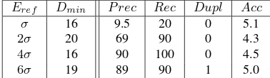
Table 3 investigates the choice of the dissimilarity normaliza-tion factorEref. ChoosingEref below2σgenerates many
Eref Dmin P rec Rec Dupl Acc
σ 16 9.5 20 0 5.1
2σ 20 69 90 0 4.3
4σ 16 90 100 0 4.5
6σ 19 89 90 1 5.0
Table 3: Results on synthetic dataset for increasing Dref withσ= 4cm,Ncam= 5
small compact clusters that do not necessarily correspond to particles (they might be coincidental with so many lines). Conversely, large values will under-segment (one reconstruc-tion for multiple particles), which lowers both precision and recall. Moreover, highErefvalues make the problem more difficult as the consistency graph becomes much denser, so it has much more cliques, which decreases the quality of the re-sult for the maximum clique computation that has a constant time budget, and increases computation time for the local op-timality.
For all the experiments, we used a time budget for maximal clique computation of 30s which proved sufficient in most cases. The computation time thus mainly depends on the lo-cal optimality computation. For 100 nodes, this computation takes from a minute to 10 for very dense graphs. For lager sizes, we recursively split and merge the component, so the computing time will be roughly linear, plus the time bud-get allocated to each merge (which are also maximum clique problems).
3.2 Application to 3D traffic sign reconstruction
To apply our methodology, we simply average the dissimi-larity from previous section over the sign corners (a specific measure should be used for circular signs). Note that the re-construction used is constrained by the shape of the 3D sign (square, equilateral triangle) in the same manner as (Soheil-ian et al., 2013). For the normalization factorEref, we esti-mate that our geroreferencing system drifts of a few centime-ters during the acquisition of images of a given sign. Given the results of previous section, we assumed that Eref = (20cm)2was a good choice.
For the discarding criterion, we used the same constraints as (Timofte et al., 2009) and (Soheilian et al., 2013):
• Geometric constraints:
– Epipolar geometry: both detected sign centers should lie on the same epipolar line of the camera pair.
– Size: the size of resulting 3D traffic sign should lie in some range (specified by a traffic sign refer-ence document).
– Visibility: the resulting 3D traffic sign should face both camera centers.
• Similarity constraint: both detected signs should have the same visual characteristics.
A B
C
Figure 4: An ambiguous clustering problem. Top: a greedy heuristic generates a "ghost" 3D signs at C when reconstruct-ing the real signs A and B. Bottom: our combinatorial clus-tering successfully removed C, reattributing all 2D detections to the correct 3D sign, also improving accuracy.
(1 False Negative) and two reconstructions had no counter-part in the ground truth (2 False Positives, against 9 with a greedy heuristic). Seven signs were duplicated. Most of the "ghost" signs from the greedy heuristic of (Soheilian et al., 2013) were eliminated as illustrated in Figure 4, validating its practical interest. Processing time (for the combinatorial clustering) was around 1 hour.
4. CONCLUSIONS
This paper proposed a general framework for combinatorial clustering that can be applied in a wide range of contexts, in particular to disambiguate the reconstruction of similar 3D objects such as traffic signs. Even if our formulation of the problem makes it hard to solve in complex cases, we pro-posed several improvements that makes it tractable on most cases that we encountered. Moreover our interlaced strategy for splitting very large problems shows good performance even if we cannot give guarantees that the resulting parti-tion is optimal. Our experiments have shown a significant improve compared to our previous greedy heuristic, with a correct handling of most ambiguities. Thus we consider that this work has overcome a significant difficulty inherent to the problem of reconstruction of similar 3D object, which may be applicable to other contexts. The major limit, inherent to the problem, is the ratio between the precision of the de-tection and the minimum distance between objects. When it becomes too high, the problem becomes too ambiguous for a correct solution to be found.
In the future, we plan on validating more finely the approx-imations necessary to make the problem tractable, but also
on refining the criteria used to create the consistency graph. For instance, we would like to make use of a 3D city model in order to predict occlusions more finely in order to have a sim-pler consistency graph. Finally, the complexity of the prob-lem could be reduced if we track the signs for each camera, in which case we would cluster not the signs but the series of signs from tracking.
ACKNOWLEDGEMENTS
This study has been performed as part of the Cap Digital Business Cluster TerraMobilita Project.
REFERENCES
Cornelis, N., Leibe, B., Cornelis, K. and Gool, L., 2008. 3D Urban Scene Modeling Integrating Recognition and Recon-struction. International Journal of Computer Vision 78(2-3), pp. 121–141.
Fang, C.-y., Member, A., Chen, S.-w., Member, S. and Fuh, C.-s., 2003. Road-sign detection and tracking. IEEE Trans-actions on Vehicular Technology 52(5), pp. 1329–1341.
Früh, C. and Zakhor, A., 2004. An automated method for large-scale, ground-based city model acquisition. Interna-tional Journal of Computer Vision 60, pp. 5–24.
Fu, M. and Huang, Y., 2010. A survey of traffic sign recogni-tion. In: International Conference on Wavelet Analysis and Pattern Recognition (ICWAPR), IEEE, pp. 119–124.
Lafuente-Arroyo, S., Maldonado-Bascon, S., Gil-Jimenez, P., Acevedo-Rodriguez, J. and Lopez-Sastre, R. J., 2007. A Tracking System for Automated Inventory of Road Signs. In: IEEE Intelligent Vehicles Symposium, Ieee, pp. 166–171.
Leonardis, A., Gupta, A. and Bajcsy, R., 1995. Segmenta-tion of range images as the search for geometric paramet-ric models. International Journal of Computer Vision 14(3), pp. 253–277.
Li, H. and Nashashibi, F., 2010. Localization for intelligent vehicle by fusing mono-camera, low-cost GPS and map data. In: Intelligent Transportation Systems, Madeira Island, Por-tugal, pp. 1657–1662.
Meuter, M., Kummert, A. and Muller-Schneiders, S., 2008. 3D Traffic Sign Tracking Using a Particle Filter. In: 2008 11th International IEEE Conference on Intelligent Trans-portation Systems, pp. 168–173.
Niskanen, S. and Östergård, P. R. J., 2003. Cliquer user’s guide, version 1.0. Communications Laboratory, Helsinki University of Technology, Espoo, Finland.
Soheilian, B., Paparoditis, N. and Vallet, B., 2013. Detec-tion and 3D reconstrucDetec-tion of traffic signs from multiple view color images. ISPRS Journal of Photogrammetry and Re-mote Sensing 77, pp. 1–20.
Timofte, R., Zimmermann, K. and Van Gool, L., 2009. Multi-view traffic sign detection, recognition, and 3D local-isation. In: 2009 Workshop on Applications of Computer Vision (WACV), IEEE, Snowbird, UT, pp. 1–8.