Directory UMM :Data Elmu:jurnal:L:Labour Economics:Vol7.Issue5.Sep2000:

(1)

www.elsevier.nlrlocatereconbase

Effects of the United States tax system on

transitions into self-employment

Donald Bruce

)

Center for Business and Economic Research and Department of Economics, UniÕersity of Tennessee,

KnoxÕille, TN 37996 4170, USA

Abstract

This paper examines the impact of US income and payroll taxes on the decision of wage-and-salary employees to become self-employed. I exploit variations in the tax treatment of wage and self-employment income using the Panel Study of Income Dynamics. Results show that differential taxation has significant effects on the probability of making a transition into self-employment. Reducing an individual’s marginal tax rate on self-em-ployment income while holding his marginal wage tax rate constant reduces the probability of entry. Conversely, reducing his relative aÕerage tax rate in self-employment increases

JEL classification: J23; H24

Keywords: Self-employment; Income taxation

1. Introduction

The number of self-employed Americans has grown steadily since the early 1970s, due largely to the increased entry of female entrepreneurs and growth in the number of independent contractors in the economy. A recent estimate finds the size of this group to be about 14 million, or 23 million if independent contractors

Ž .

are counted Pink, 1998 . Drawing upon data from the US Current Population

Ž .

Surveys, Schuetze 1998 notes that the self-employment rate among American prime-age males was 12.4% in 1994. While growing bodies of research have

)_Tel.:_q_{1-865-974-6088; fax:}_q_{1-856-974-3100.}

Ž .

E-mail address: dbruce@utk.edu D. Bruce .

Ž .

(2)

( ) D. BrucerLabour Economics 7 2000 545–574

546

documented the dynamics of self-employment as well as various behavioral effects of taxation, the effects of taxes on self-employment have received relatively little attention.

Differential tax treatment could affect the decision to become self-employed in

Ž .

various ways, two examples of which were noted by Goode 1949 . First, the taxation of self-employment income depends on voluntary compliance, while most of the wage-and-salary tax payments are withheld by employers. Second, many expenses related to self-employment are deductible in calculating taxable income. These two factors represent conditions that might pull potential entrepreneurs into self-employment. More generally, tax changes could change self-employment rates by making self-employment relatively more or less attractive than wage-and-salary work. Such effects might include a general increase in taxes, such as rate increases or base-broadening measures, which might push workers out of wage-and-salary jobs.

Some important changes in the relative tax treatment of these two types of work occurred during the 1980s that made self-employment much less tax-advantaged than it had previously been. It is the goal of this study to use this variation in relative tax treatment to estimate the incentive or disincentive effects of the US income and payroll tax systems on self-employment start-ups. If the tax system is indeed discouraging entrepreneurship, the resulting misallocation of productive inputs away from self-employment causes economic inefficiency. However, if the original tax advantages bestowed upon the self-employed were misguided, the recent changes could represent an overdue correction. While I do not attempt to estimate the socially optimum number of self-employed workers, I do examine the relative responsiveness to tax changes among those potentially considering en-trepreneurship.

The remainder of the paper is organized as follows. Section 2 provides a brief history of the differential tax treatment of the self-employed. Section 3 reviews the existing empirical literature on taxes and self-employment and Section 4 describes the data and empirical strategy used. Empirical findings are presented in Section 5, with conclusions and suggestions for further research in Section 6.

To anticipate the primary results, I find that taxes have significant effects on the probability that an individual will leave a wage-and-salary job to become self-em-ployed. The most robust estimates indicate that a five percentage point increase in

Ž .

the wage-and-salary minus self-employment difference between an individual’s expected marginal tax rates reduces his transition probability by about 2.4 percentage points.

2. A history of the differential tax treatment of the self-employed

Since their inception, the US income and payroll tax systems have treated income from wage-and-salary and self-employment differently. This distinction

Ž .

(3)

process for the self-employed. While wage-and-salary workers have both income and payroll taxes withheld by their employers, the self-employed must assume this responsibility individually.

Income from wage-and-salary employment has been subject to a payroll tax since 1937, its proceeds serving as the primary funding for the Social Security

Ž

system. Generally, a percentage of a worker’s earnings up to some maximum .

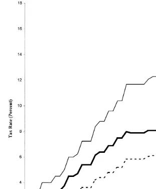
taxable amount is withheld, and that percentage is matched by the employer. Self-employment income was not subject to a payroll tax until 1951. From 1951 through the early 1960s, the statutory payroll tax rate on self-employment income was one-and-a-half times the employee’s rate on wage-and-salary income. From the early 1960s through 1984, however, self-employment income was subject to a tax that was less than one-and-a-half times the wage-and-salary rate. Fig. 1 shows

Ž

the net statutory payroll tax rates for wage-and-salary combined and employer

. 1

alone and self-employed individuals.

Beginning in 1984, in an effort to equalize the treatment of wage-and-salary and self-employment income, the statutory self-employment payroll tax rate was set equal to two times the wage-and-salary rate. Essentially, self-employed indi-viduals were made liable for payroll taxes equal to the employer and employee shares for wage-and-salary individuals. While tax credits were used to phase in the change from 1984 to 1990, this series of events represents a dramatic change in the relative tax treatment of self-employment income.

Coupled with these changes in the payroll tax system during the 1980s was a significant, although perhaps less dramatic, change in the relative income tax treatment of wage-and-salary and self-employed individuals. For both categories of workers, tax rates were reduced and the tax base was increased. For the self-employed, a number of limitations on deductible business expenses were passed. Other fringe benefits, often paid for in wage-and-salary jobs out of pre-tax dollars, are still not deductible in self-employment. Further, before 1987, the self-employed could not deduct health insurance costs on their income tax returns. Conversely, more liberal provisions relating to the business use of one’s home made self-employment relatively more attractive during this time.

Despite some small gains, the payroll and income tax changes during the 1980s rendered self-employment significantly less tax-advantaged relative to wage-and-salary employment. Indeed, the overall theme of the 1980s tax changes was to level the playing field for various types of taxpayers. These changes in the Federal

1

ByAnetBstatutory payroll tax rates, I mean inclusive of the phase-in credits and exclusion amounts mentioned in the text. In a further effort to equalize the treatment of wage-and-salary and self-employ-ment income, as of 1990 the self-employself-employ-ment payroll tax applies to only 92.35% of self-employself-employ-ment earnings, and half of the self-employment taxes due may be deducted in the computation of adjusted

Ž .

gross income AGI . The gross, pre-credit, statutory social security tax rates for wage-and-salary

(4)

548

Fig. 1. Payroll tax rates, 1950–1995.

tax code-along with substantial variation at the state and individual levels-provide ample variation that can be used in analyzing individual sensitivity to taxes among potential entrepreneurs.

3. A review of the empirical literature

(5)

on self-employment rates. A few have analyzed individual-level cross-sectional data, but most have used aggregated tax variables to avoid the potential endogene-ity of taxes on the individual level; only two of these used individual-level tax information, and neither one tested or corrected for the endogeneity of tax rates.

Ž .

Beginning with the time-series studies, Long 1982a investigated the effects of income tax rates on the SMSA-level ratio of self-employment to total employment. Using 1970 Census data, he found that a 10% increase in the average marginal income tax rate in an SMSA increased the self-employment rate in that SMSA by 6.4%. Further, a US$300 increase in average income tax liability increased the self-employment rate by 1%.

Ž . Ž .

Blau 1987 followed Long’s 1982a method and estimated aggregate time-series regressions using US data for 1948 through 1982. His tax variables consisted of two marginal tax rates, however, for incomes of US$7000 and US$17,000, respectively. While his findings at the higher marginal tax rate supported Long’s, Blau found that increases in lower-bracket marginal tax rates actually reduced the self-employment rate. This empirical puzzle was not ex-plained.

Ž . Ž .

Parker 1996 more closely resembled Long 1982a , but used a 1959 to 1991 time series of United Kingdom data. Again, higher marginal tax rates were found

Ž .

to increase self-employment rates. He followed Blau 1987 in using two marginal tax rates associated with two different levels of income, but failed to support Blau’s findings at the lower rate.

Ž .

Robson and Wren 1998 provided a theoretical model that incorporated both average and marginal tax rates. Their model predicted, and time-series regressions confirmed, that higher average tax rates reduced self-employment rates while higher marginal tax rates increased self-employment. This divergence was at-tributed to the assumptions that self-employment earnings more closely resemble

Ž

the value of the individual’s marginal product of labor i.e., a higher average tax .

rate in self-employment reduces the net reward from working , and that higher marginal tax rates increase the payoff to evading or avoiding taxes by under-re-porting income or increasing business-related deductions.

This time-series evidence on taxes and self-employment supports the popular claim that individuals become self-employed in order to avoid paying higher wage-and-salary taxes. However, the most recent time-series evidence, presented

Ž .

by Fairlie and Meyer 1998 , finds no significant effect of taxes on self-employ-ment rates. Using aggregated individual data from seven decennial Censuses of

Ž .

Population for 1910 and 1940–1990 , they found that the overall relationship between tax rates and self-employment is, at best, weak during this period. Their paper is an exception, however, as no multivariate analysis was performed to test this conclusion.

Cross-sectional evidence generally supports the earlier time-series results. Long

Ž1982b used disaggregated data from the 1970 Census for males between the ages.

(6)

550

regressed on expected income tax liability under wage-and-salary employment indicated economically and statistically significant tax effects. Echoing his aggre-gate findings, an increase in expected wage-and-salary tax liability of 10% was found to increase the probability of being self-employed by 7.4%.

Ž .

Moore 1983 expanded on Long’s research, but focused on the payroll tax.

Ž .

Indeed, Moore’s was the first and only study to examine both individual income and the payroll taxes using microdata. He used 1978 CPS data for males between 25 and 65 working full time to estimate linear probability models and logits of self-employment status. The effect of the expected wage-and-salary income tax

Ž .

variable was significant, but much smaller than those estimated by Long 1982a,b . Moore found much larger effects from the payroll tax; a 10% increase in expected wage-and-salary payroll tax liability caused a 5 to 8% increase in the probability of being self-employed.

Ž .

Schuetze 1998 provided the most recent look at the effects of taxes on

self-employment, using aggregate Atax climateB variables in a cross-sectional

comparison of the United States and Canada. Using CPS data for 1983 through 1994, he found that a 10% increase in the US average marginal tax rate in one year caused a 2.1% increase in the probability of being self-employed in the following year.2

While these studies conclude almost universally that higher overall marginal tax rates increase self-employment rates, they do not actually estimate individual-level sensitivity to the relative tax treatment of the self-employed. Two recent papers by

Ž .

Carroll et al. 1995, 1997 provided evidence of the importance of investigating the tax response using individual-level data. Their investigation of the impact of taxes on decisions by existing entrepreneurs to hire additional workers and make capital investments suggests that the self-employed are indeed cognizant of their own personal tax situations. Specifically, marginal tax rate increases were found to reduce both mean investment expenditures and the probability of hiring employ-ees.

While individual-specific taxes have been found to have important effects on the actions of those already in self-employment, little is known about their effects on entry into self-employment. It is the intent of this paper to examine whether or not indiÕidual-leÕel income and payroll taxes affect indiÕidual decisions to

become self-employed. More precisely, I wish to estimate the existence of tax effects by examining the expected post-transition tax situations of potential entrepreneurs during the 1980s. Also, in order to correctly gauge the level of tax sensitivity, I focus on individual-specific tax differentials by comparing each person’s tax situation in wage-and-salary and self-employment.

2

(7)

4. Data and empirical specification

I follow a number of earlier self-employment transition analyses in developing an empirical strategy to estimate these effects.3 _{Specifically, I estimate equations}

of the following type:

D sbX

X qgT qm qn ,

Ž .

1

i , tq1 i , t i , tq1 i i , tq1

where Di, tq1 is a dummy variable that equals one if individual i moves from

wage-and-salary at time t to self-employment at time tq1, and zero if he remains

wage-and-salary in both periods. The Xi, t vector includes a constant term and a

set of time t exogenous variables, and the Ti, tq1 term represents the individual-specific difference in wage-and-salary and self-employment tax rates at time tq1.

The error term in this equation includes an individual-specific time-invariant

Ž .

random effect mi to capture unobserved individual heterogeneity, and an

inde-Ž .

pendently and identically distributed residual component Õ with zero mean

i, tq1

Ž .

and finite variance. A convenient empirical specification for Eq. 1 is a random effects probit.

It should be noted that the use of tax rates as opposed to tax levels, or liabilities, is somewhat arbitrary. The two are certainly correlated, but equal tax

Ž .

rates where the difference in the rates equals zero will have the same effect in the multivariate analysis regardless of the levels of tax liabilities. At the heart of

Ž .

this situation is the issue of tax evasion or avoidance. Joulfaian and Rider 1998 have found a positive relationship between marginal tax rates and tax evasion

Ž .

among the self-employed, and Blumenthal et al. 1998 have shown that Schedule

Ž .

C filers for self-employment income are significantly more likely to evade taxes.

Ž .

Consequently, it would be preferential but highly difficult to control for this type of behavior.

By assuming full compliance on the part of the self-employed for the purposes of this study, I am measuring the benefit from noncompliance by the tax rate rather than the actual dollar value, or tax liability. As it is expected that rates and

Ž

levels are highly correlated and that either, when implemented as differences from wage-and salary rates or liabilities, would capture the payoff to evasion and

.

avoidance , I use rates for purposes of comparison to all but the three earliest empirical studies in this literature.4

3

Transition analysis offers the important advantage over cross-sectional analysis of being able to date the explanatory variables in the pre-transition period, thus avoiding problems of potential endogeneity. Further, previous research has found that empirical results are very similar in both types

Ž .

of studies see, for example, Meyer, 1990 . 4

(8)

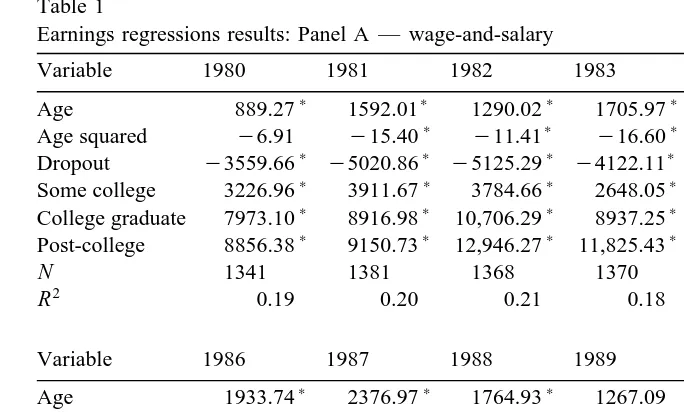
552 Table 1

Earnings regressions results: Panel A — wage-and-salary

Variable 1980 1981 1982 1983 1984 1985

) ) ) ) ) )

Age 889.27 1592.01 1290.02 1705.97 1524.42 2394.51

) ) ) ) )

Age squared y6.91 y15.40 y11.41 y16.60 y13.20 y24.45

) ) ) ) ) )

Dropout y3559.66 y5020.86 y5125.29 y4122.11 y4749.21 y5615.76

) ) ) ) ) )

Some college 3226.96 3911.67 3784.66 2648.05 2958.97 3560.44

) ) ) ) ) )

College graduate 7973.10 8916.98 10,706.29 8937.25 11,595.03 10,387.91

) ) ) ) ) )

Post-college 8856.38 9150.73 12,946.27 11,825.43 12,756.87 13,571.03

N 1341 1381 1368 1370 1403 1448

2

R 0.19 0.20 0.21 0.18 0.20 0.19

Variable 1986 1987 1988 1989 1990 1991

) ) ) )

Age 1933.74 2376.97 1764.93 1267.09 1449.30 2298.25

) )

Age squared y17.97 y23.19 y15.18 y8.48 y10.43 y22.52

) ) ) ) )

Dropout y6036.67 y5060.52 y5665.47 y6765.12 y5636.81 y5186.47

) ) ) ) ) )

Some college 5093.06 5488.82 4929.59 4695.14 4622.51 5364.25

) ) ) ) ) )

College graduate 12,226.74 14,761.83 13,460.71 13,754.43 14,976.37 16,836.97

) ) ) ) ) )

Post-college 15,980.23 19,233.98 21,367.32 24,603.75 25,878.29 29,834

N 1493 1548 1553 1593 1601 1600

2

R 0.22 0.22 0.20 0.20 0.19 0.13

Entries are OLS regression coefficients. Regressions also include a constant term. The dependent variable is the head’s labor earnings in dollars.

)_{Statistically significant at the 5% level.}

Of course, I only observe one actual tax rate-either in wage-and-salary or in self-employment-for each individual in each year depending on which sector is actually chosen. Consequently, I estimate each individual’s labor earnings in the alternative sector for each time period. Earnings regressions of the following form are estimated for each sector in each year:

YWS_sa_Z _q_{e ,}

_{Ž .}

₂

i , t i , t i , t

YSE

sfZ qf ,

Ž .

3

i , t i , t i , t

where Y is gross labor income, i indexes individuals, and t indexes time. Z_{i, t}

Ž consists of measures for age and educational attainment, and the error terms e_{i, t}

. 5

and f_{i, t} are normally distributed with zero mean and finite variance. The

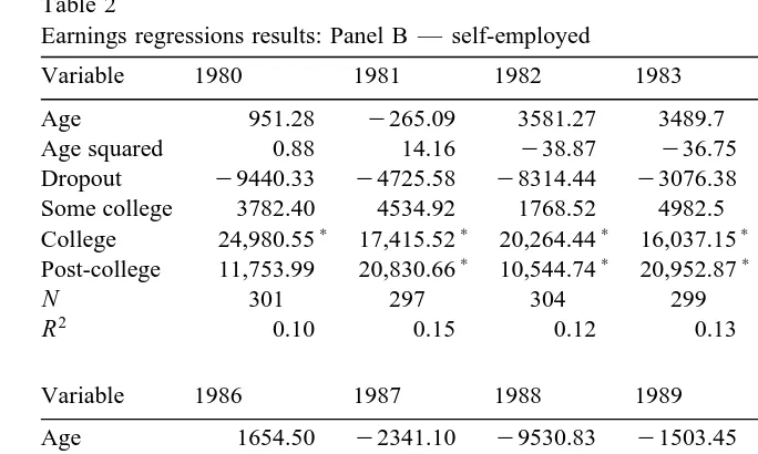
coefficients from these regressions are then used to predict wage-and-salary

Ž .

earnings for self-employed individuals, and vice versa Tables 1 and 2 . I use these predicted income figures together with the National Bureau of Economic Research

5

(9)

Table 2

Earnings regressions results: Panel B — self-employed

Variable 1980 1981 1982 1983 1984 1985

Age 951.28 y265.09 3581.27 3489.7 5564.08 6284.93

Age squared 0.88 14.16 y38.87 y36.75 y64.28 y70.77

Dropout y9440.33 y4725.58 y8314.44 y3076.38 y2595.45 y4367.88

Some college 3782.40 4534.92 1768.52 4982.5 3449.65 965.74

) ) ) ) ) )

College 24,980.55 17,415.52 20,264.44 16,037.15 17,660.95 20,980.68

) ) ) ) )

Post-college 11,753.99 20,830.66 10,544.74 20,952.87 36,264.58 33,268.97

N 301 297 304 299 318 312

2

R 0.10 0.15 0.12 0.13 0.13 0.13

Variable 1986 1987 1988 1989 1990 1991

)

Age 1654.50 y2341.10 y9530.83 y1503.45 8337.04 6137.39

)

Age squared y10.78 45.64 137.97 30.59 y99.46 y69.94

Dropout y10,159.8 y9889.13 y8158.59 y3684.45 y6017.81 y7499.61 Some college 556.09 5559.45 10,011.71 3745.37 9567.65 6991.68

) ) ) ) )

College 20,221.81 39,409.85 44,846.52 32,118.31 18,350.6 18,357.24

) ) ) ) ) )

Post-college 36,609.22 31,747.14 33,295.13 47,134.93 55,825.86 67,923.81

N 305 313 322 329 320 327

2

R 0.16 0.06 0.07 0.09 0.18 0.15

Entries are OLS regression coefficients. Regressions also include a constant term. The dependent variable is the head’s labor earnings in dollars.

)_{Statistically significant at the 5% level.}

ŽNBER TAXSIM model to calculate predicted alternative-sector tax rates, and.

their difference from the actual tax rates, in each year. I also calculate payroll tax liability and include it in all tax rate calculations.6

Consider, for example, the case of a wage-and-salary individual who becomes Ž

self-employed in the next survey year. His post-transition earnings in self-em-.

ployment are observed, and his actual taxes and rates can be predicted using the TAXSIM program. In order to investigate differential taxation, however, his hypothetical earnings and taxes in wage-and-salary must be estimated. After this prediction procedure is complete, I have two sets of earnings and tax data for this and all other individuals that are then used to create necessary tax differentials for the empirical analysis. An in-depth discussion of the tax rate calculation process is provided in Appendix A.

6

Payroll taxes might be expected to have smaller effects on transition probabilities, primarily because the payment of Social Security and Medicare taxes is associated with clearly defined benefits. Higher payroll tax rates will typically carry higher benefits, albeit on a less than one-for-one basis. It should be noted, however, that the time period in this analysis is characterized by rate increases for the self-employed relative to wage-and salary workers without equivalent relative benefit increases. Indeed,

Ž .

(10)

554

An important issue to address is the potential endogeneity of the tax rate differential in the above transition probit. Whether or not an individual moves from wage-and-salary to self-employment will certainly have some effect on his calculated tax rate differential. To control for this endogeneity, I use the instru-mental variables approach suggested in the study of tax reforms and investment by

Ž . Ž .

Cummins et al. 1994 and later used by Carroll et al. 1995, 1997 .

Specifically, I compute two separate tax rate differentials for each t to tq1

transition. The first, discussed above, uses tq1 incomes and tax rules and

represents the closest approximation to the actual differential. Each individual’s post-transition tax rate differential is a function of all observable and unobservable individual behavior, however, which makes it potentially endogenous. The second,

hypothetical differential uses time tq1 income under the time t tax rules. The

TAXSIM model allows this approach to be implemented quite easily. The hypothetical differential captures the difference in tax rates that would have existed had the tax rules remained constant. The instrumental variable is then equal to the difference in these two tax rate differentials, and represents the part of the actual differential that is caused by the change in the tax code only; the part that is a result of individual behavior is subtracted out of the actual differential. Because of the two-period design of the statistical analysis, panel data is required. My initial sample consists of data from the 1970 through 1991 waves of

Ž .

the Panel Study of Income Dynamics PSID . TAXSIM can only be used to estimate tax rates beginning in 1979, however, so I focus on transitions beginning in the years 1979 through 1990. This rich panel data set provides ample informa-tion on individual, household, and occupainforma-tional characteristics. Further, sample sizes for self-employed individuals are large enough to permit longitudinal analy-sis of the start-up decision. Yearly self-employed sample sizes are often small enough, however, that some form of pooled data analysis is preferred.

Following much of the existing empirical literature, I confine the analysis to male heads of household who are between the ages of 25 and 54. The dynamics of self-employment are likely to be quite different among younger and older

individ-uals and among females.7 _{The head-of-household restriction is a direct result of}

the fact that the PSID provides self-employment status for household heads and their spouses only. These assumptions leave a sample of 2638 individuals with at least 1 year of data on self-employment status.

For the purposes of this study, an individual is considered to be self-employed if he reports working for himself or for himself and someone else at the time of the survey. This latter category is minimal-usually less than 1% of the working

7

A number of other studies have analyzed self-employment for these groups. For example, Fuchs

Ž1982 examines self-employment among older individuals. Dunn and Holtz-Eakin forthcoming and. Ž .

Ž . Ž . Ž .

Blanchflower and Meyer 1994 consider younger individuals. Devine 1994 , MacPherson 1988 , and

Ž .

(11)

sample in each year. These individuals are kept in order to increase sample sizes and to capture all experiences in self-employment.8

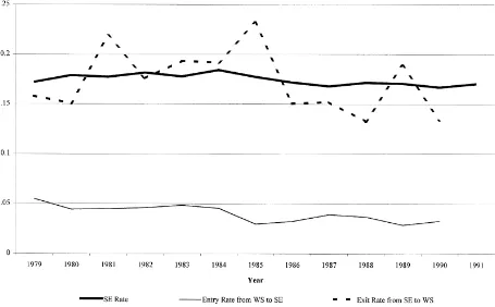
Fig. 2 shows self-employment rates for the sample of 2638 men from 1979 to 1991. The self-employment rate is fairly constant over time for this group, usually between 17% and 18%. Fig. 2 also presents transition rates from wage-and-salary to self-employment over time. Despite fairly constant self-employment rates, the transition rate from wage employment to self-employment shows a noticeable decline over time for this sample. The rate of exit from self-employment to wage employment partially explains these seemingly incompatible trends. However, Fig.

Ž

2 shows an exit rate that seems to trend upward during the early 1980s perhaps in .

response to eroding tax advantages , but then declines, albeit in a rather volatile manner, contributing to the fairly constant self-employment rate. Nonetheless, the

reduction in the taxApayoffB to becoming self-employed may be one of the many

factors at work in the downturn in entry rates during the 1980s.

For an individual to be in the sample used to estimate the transition probit, he must be wage-and-salary in the first period and either wage-and-salary or self-em-ployed in the next period, and he must be out of school. Consequently, I have a select sample; those who are already in self-employment cannot enter the analysis. To be more precise, the individuals in the transition probit have not yet made an observable transition into self-employment, or, if they entered before they were first observed in the data, they returned to wage-and-salary work at some point before the period of analysis. The data-screening process removes those who start in self-employment and never leave. Therefore, the individual random effect — which is intended to capture unobserved entrepreneurial ability — is potentially correlated with the transition indicator. This is a case of the so-called initial conditions problem.

To correct for this type of potential bias, I follow the method suggested by

Ž .

Orme 1997 . This procedure essentially allows the initial conditions problem to be converted into a more tractable sample selection problem. The first stage of this procedure is a probit regression of a dummy variable that takes the value of one if the man is first observed in a wage-and-salary job and zero if he is first observed in self-employment. Regressors consist of a set of individual, household, and regional characteristics in the year he is first observed. Note that each individual’s

Ž

initial observation may come from any year during the panel period 1970 through .

1990 if the individual happens to be in school or out of the labor force in the first

8

Concerns have been raised in many studies about the appropriateness of screening a self-employed sample on the basis of earnings or hours worked. Such a procedure would supposedly eliminate the

Apartially self-employedB or those claiming to be fully self-employed but who in fact are not really

Ž .

(12)

()

D.

Bruce

r

Labour

Economics

7

2000

545

–

574

556

(13)

panel year. Identification of this stage is accomplished by including veteran status as a regressor, which does not appear later in the transition equations.

Ž .

In order for Orme’s 1997 procedure to be appropriate in this case, however, individuals who are either self-employed in their initially observed occupation or have entered self-employment at some previous point in the panel period must be omitted from the transition probits. This leaves a sample of initially wage-and-salary workers who will be followed until they either make a single transition into self-employment, they drop out of the survey, or they reach the end of the panel

Ž .

period. In a simplification of Orme’s 1997 procedure, an inverse Mills ratio is calculated using the estimates of the first-stage probit.9 _{This Mills ratio is included}

as a regressor in the random effects transition probit, along with a similar set of individual, household, and regional characteristics.

Approximately 11% of the individuals in the initial sample are self-employed in their first observed jobs. Only about 26% of all first jobs actually occur in 1970, the first year in my sample. The remaining 74% are distributed nearly evenly over the years from 1971 to 1990, indicating that I observe actual initial conditions for the majority of the sample. When I look only at those who make at least one transition from wage-and-salary to self-employment, slightly less than 10% are self-employed in their first job.

Next, looking at the remaining sample of those who were initially wage-and-salary and eliminating multiple transitions leaves a total sample of 206 first observable transitions to analyze. However, a few of these individuals do not report information for one or more of the various control variables, which restricts the actual regression sample size to 1193 individuals, 184 of whom eventually

make a transition into self-employment.10 _{Pooling the observations from these}

1193 individuals over the period from 1979 to 1990 yields a final sample of 5622 person-years of usable data for the transition analysis.

Again, I follow previous studies of transitions into self-employment in selecting a set of control variables to include in X . Individual characteristics include agei, t

Ž_{in quadratic form , a set of indicators for educational attainment of less than high}.

Ž . Ž . Ž

school 11 or fewer years , some college between 13 and 15 years , college 16

. Ž .

years , and post-college more than 16 years , and an indicator for nonwhite race. Household-level controls include marital status, entered as a dummy variable for married, and a series of continuous variables for the number of children in the household in various age groups.

9 _Ž _.

Orme’s 1997 procedure is designed to allow observations coming from more than one initial condition to enter the final stage of the estimation process.

10 _Ž _.

Fitzgerald et al. 1998 examine the impact of sample attrition on the representativeness of the PSID, concluding that attrition is not generally a serious problem. While I have not repeated their procedure to gauge the impact of attrition as it relates to self-employment, it is not clear whether my reduced sample should be representative of any particular population. For this reason, none of the

Ž .

(14)

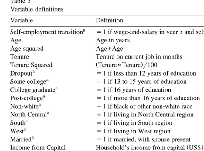
558 Table 3

Variable definitions

Variable Definition

a

Self-employment transition s1 if wage-and-salary in year t and self-employed in year tq1

Age Age in years

Age squared Age)Age

Tenure Tenure on current job in months

Ž .

Tenure Squared Tenure)Tenurer100

a

Dropout s1 if less than 12 years of education a

Some college s1 if 13 to 15 years of education a

College graduate s1 if 16 years of education a

Post-college s1 if more than 16 years of education a

Non-white s1 if black or other non-white race a

North Central s1 if living in North Central region a

South s1 if living in South region

a

West s1 if living in West region

a

Married s1 if married, with spouse present

Ž .

Income from Capital Household’s income from capital US$1000 a

Part-Time s1 if worked between 52 and 1820 annual hours

Kids 1 to 2 Number of children in the household between the ages of 1 and 2 Kids 3 to 5 Number of children in the household between the ages of 3 and 5 Kids 6 to 13 Number of children in the household between the ages of 6 and 13 Kids 14 to 17 Number of children in the household between the ages of 14 and 17

a

Union s1 for membership in a labor union

Unemployment rate County unemployment rate a

MSA s1 if living in a metropolitan statistical area When not otherwise indicated, all variables represent information at year t.

a

Dummy variable.

As a transition into self-employment carries certain opportunity costs, I also

Ž .

include a set of job-specific controls. These consist of tenure in months on the current wage-and-salary job entered in quadratic form, and dummies for part-time employment and union membership in the pre-transition year. Regional and macroeconomic effects are controlled for via a set of indicators for residence in the north-central, south, and west regions, a dummy for whether or not the

Ž .

individual lives in a metropolitan statistical area MSA , and the local area

Ž_{county unemployment rate. Dummy variables for the year of the observation are}.

included to control for other potential time-related effects.

A number of studies have found that greater wealth holdings increase the likelihood of a transition into self-employment.11_{This is consistent with the notion}

11 _Ž _. _Ž _. _Ž _.

Evans and Leighton 1989 , Evans and Jovanovic 1989 , and Meyer 1990 are among the

Ž .

pioneering studies of liquidity constraints and self-employment. Blanchflower and Oswald 1998 and

Ž .

Holtz-Eakin et al. 1994a,b also reveal the importance of available financial capital to self-employ-ment entry and duration. While I do not specifically include spouse’s income as a control, it is included

Ž .

(15)

that liquidity constraints are present. While the PSID does not include a yearly wealth variable, it does have the household’s yearly income from capital. This will

Ž .

presumably be positively correlated with the household’s unobserved total

wealth holdings, so it is used here as a proxy.

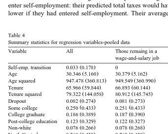
Table 3 provides definitions of these control variables, and Table 4 presents descriptive statistics for the regression sample. Individuals making a transition into self-employment are, before the transition, slightly younger than those who do not enter self-employment. They have also worked fewer months on their wage-and-salary job, are more likely to be white, are more likely to be working part time, and are much less likely to belong to a union.

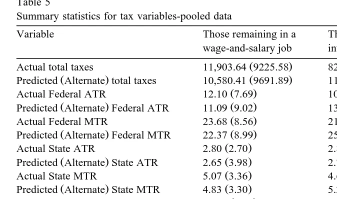
Table 5 provides a preliminary look at the actual and hypothetical post-transi-tion tax situapost-transi-tions for the regression sample. Looking first at those who do not enter self-employment: their predicted total taxes would have been nearly US$1500 lower if they had entered self-employment. Their average and marginal tax rates

Table 4

Summary statistics for regression variables-pooled data

Variable All Those remaing in a Those making a transition

wage-and-salary job into self-employment

Ž .

Self-emp. transition 0.033 0.178 0 1

)

Ž . Ž . Ž .

Age 30.346 5.160 30.379 5.162 29.348 5.012

)

Ž . Ž . Ž .

Age squared 947.478 360.813 949.549 360.990 886.283 351.004

)

Ž . Ž . Ž .

Tenure 65.966 59.844 66.893 60.144 38.587 41.864

)

Ž . Ž . Ž .

Tenure squared 79.322 144.058 80.912 145.745 32.320 63.588

Ž . Ž . Ž .

Dropout 0.082 0.274 0.081 0.273 0.109 0.312

Ž . Ž . Ž .

Some college 0.250 0.433 0.251 0.433 0.223 0.417

Ž . Ž . Ž .

College graduate 0.186 0.389 0.187 0.390 0.174 0.380

Ž . Ž . Ž .

Post-college education 0.123 0.329 0.122 0.327 0.168 0.375

)

Ž . Ž . Ž .

Non-white 0.076 0.266 0.078 0.268 0.043 0.204

Ž . Ž . Ž .

North Central 0.260 0.439 0.260 0.439 0.255 0.437

Ž . Ž . Ž .

South 0.304 0.460 0.305 0.460 0.266 0.443

Ž . Ž . Ž .

West 0.200 0.400 0.198 0.399 0.250 0.434

Ž . Ž . Ž .

Married 0.835 0.371 0.834 0.372 0.859 0.349

Ž . Ž . Ž .

Income from capital 0.729 2.675 0.735 2.704 0.531 1.603

)

Ž . Ž . Ž .

Part-time 0.143 0.350 0.141 0.348 0.212 0.410

Ž . Ž . Ž .

Kids 1 to 2 0.338 0.550 0.338 0.550 0.337 0.559

)

Ž . Ž . Ž .

Kids 3 to 5 0.290 0.530 0.286 0.525 0.418 0.639

Ž . Ž . Ž .

Kids 6 to 13 0.398 0.752 0.399 0.751 0.359 0.769

)

Ž . Ž . Ž .

Kids 14 to 17 0.071 0.318 0.072 0.321 0.027 0.194

)

Ž . Ž . Ž .

Union 0.206 0.405 0.211 0.408 0.076 0.266

)

Ž . Ž . Ž .

Unemployment rate 6.283 2.753 6.298 6.298 5.832 2.431

Ž . Ž . Ž .

MSA 0.573 0.495 0.574 0.574 0.543 0.499

N 5622 5438 184

Entries are means, with standard deviations in parentheses. Observations are person-years.

)_{A two-tailed t test rejects the null hypothesis of equal means for columns 2 and 3 at the 5%}_Ž _.

(16)

560 Table 5

Summary statistics for tax variables-pooled data

Variable Those remaining in a Those making a transition

wage-and-salary job into self-employment

Ž . Ž .

Actual total taxes 11,903.64 9225.58 8262.28 10,529.33

Ž . Ž . Ž .

Predicted Alternate total taxes 10,580.41 9691.89 11,641.88 8825.72

Ž . Ž .

Actual Federal ATR 12.10 7.69 10.98 13.18

Ž . Ž . Ž .

Predicted Alternate Federal ATR 11.09 9.02 13.22 7.80

Ž . Ž .

Actual Federal MTR 23.68 8.56 21.47 9.78

Ž . Ž . Ž .

Predicted Alternate Federal MTR 22.37 8.99 25.75 8.96

Ž . Ž .

Actual State ATR 2.80 2.70 2.81 7.82

Ž . Ž . Ž .

Predicted Alternate State ATR 2.65 3.98 2.72 2.10

Ž . Ž .

Actual State MTR 5.07 3.36 4.61 3.38

Ž . Ž . Ž .

Predicted Alternate State MTR 4.83 3.30 5.23 3.63

Ž . Ž .

Actual payroll ATR 12.60 5.04 9.76 8.62

Ž . Ž . Ž .

Predicted Alternate payroll ATR 11.22 6.87 11.55 4.43

Ž . Ž .

Actual payroll MTR 12.73 4.77 11.02 3.60

Ž . Ž . Ž .

Predicted Alternate payroll MTR 10.09 5.30 13.68 2.91

Ž . Ž .

Total ATR differential 2.91 9.68 4.96 10.12

Ž . Ž .

Total MTR differential 4.11 8.91 7.26 9.43

Ž . Ž .

Net-of-tax income differential 971.11 10,887.76 4214.60 8018.64

Entries are means, with standard deviations in parentheses. Differential variables are calculated as the

Žactual or predicted. value under wage-and-salary minus the Žactual or predicted. value under self-employment. See text for additional details.

ATRsAverage Tax Rate. MTRsMarginal Tax Rate.

would all have been lower in self-employment. A similar pattern emerges for those who make a transition into self-employment. Their actual total tax payments are, on average, nearly US$3400 lower than they would have been had they remained in their wage-and salary job. Further, all tax rates except the state-level average tax rate are lower in self-employment than they would have been in wage-and-salary.

The last three rows of Table 5 provide summary statistics for the differential variables used in the probits. If taxes affect the probability of becoming self-em-ployed, we might expect to find that those who stand to gain the most from self-employment in terms of lower tax rates or liabilities are also the most likely to enter self-employment. A second possibility is that those whose tax rates would be higher in self-employment would be most likely to enter in order to capture the increased benefits from a given level of business-related deductions. It is the first

Ž

of these possibilities that is observed in Table 5. The total federal and state .

income plus payroll average and marginal tax rates in wage-and-salary exceed the corresponding total rates in self-employment for both categories of individuals, but by a greater amount for those who make a transition into self-employment.

(17)

have earned US$971 less on average had they entered, those who make a transition would have earned an average of US$4215 more if they had remained in a wage-and-salary job. This larger difference could be interpreted as the implicit value of the nonpecuniary benefits in self-employment.

5. Results and discussion

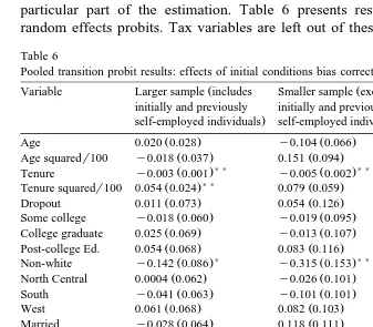
Since this is the first empirical study of self-employment transitions to attempt to control for initial conditions bias, it is useful to first gauge the impact of this particular part of the estimation. Table 6 presents results from three separate random effects probits. Tax variables are left out of these probits for the purpose

Table 6

Pooled transition probit results: effects of initial conditions bias correction

Ž Ž

Variable Larger sample includes Smaller sample excludes Smaller sample initially and previously initially and previously with correction

. .

self-employed individuals self-employed individuals

)

Ž . Ž . Ž .

Age 0.020 0.028 y0.104 0.066 y0.091 0.052

Ž . Ž . Ž .

Age squaredr100 y0.018 0.037 0.151 0.094 0.122 0.077

) ) ) ) ) )

Ž . Ž . Ž .

Tenure y0.003 0.001 y0.005 0.002 y0.006 0.001

) ) )

Ž . Ž . Ž .

Tenure squaredr100 0.054 0.024 0.079 0.059 0.084 0.046

Ž . Ž . Ž .

Dropout 0.011 0.073 0.054 0.126 0.031 0.124

Ž . Ž . Ž .

Some college y0.018 0.060 y0.019 0.095 y0.014 0.096

Ž . Ž . Ž .

College graduate 0.025 0.069 y0.013 0.107 0.010 0.104

Ž . Ž . Ž .

Post-college Ed. 0.054 0.068 0.083 0.116 0.114 0.105

) ) ) ) )

Ž . Ž . Ž .

Non-white y0.142 0.086 y0.315 0.153 y0.283 0.141

Ž . Ž . Ž .

North Central 0.0004 0.062 y0.026 0.101 y0.030 0.104

Ž . Ž . Ž .

South y0.041 0.063 y0.101 0.101 y0.106 0.098

Ž . Ž . Ž .

West 0.061 0.068 0.082 0.103 0.067 0.095

Ž . Ž . Ž .

Married y0.028 0.064 0.118 0.111 0.100 0.095

Ž . Ž . Ž .

Income from capital 0.004 0.003 y0.006 0.015 y0.011 0.012

) )

Ž . Ž . Ž .

Part-time 0.094 0.053 0.142 0.093 0.140 0.084

Ž . Ž . Ž .

Kids 1 to 2 0.029 0.042 y0.057 0.068 y0.049 0.063

) ) ) ) ) )

Ž . Ž . Ž .

Kids 3 to 5 0.076 0.039 0.225 0.065 0.244 0.059

Ž . Ž . Ž .

Kids 6 to 13 0.027 0.025 0.035 0.058 0.050 0.053

)

Ž . Ž . Ž .

Kids 14 to 17 y0.004 0.037 y0.206 0.164 y0.206 0.115

) ) ) ) ) )

Ž . Ž . Ž .

Union y0.330 0.056 y0.480 0.114 y0.383 0.109

) ) ) ) ) )

Ž . Ž . Ž .

Unemployment rate y0.020 0.008 y0.047 0.015 y0.047 0.012

Ž . Ž . Ž .

MSA y0.052 0.042 y0.048 0.075 0.017 0.077

)

Ž .

Mills Ratio – – 0.958 0.506

N 16,026 5622 5622

Sample transition 0.039 0.033 0.033

probability

Ž .

Entries are random-effects probit coefficients with robust and bootstrapped, for column 3 standard errors in parentheses. Regressions also include indicators for the year of the observation and a constant term.

(18)

562

of isolating the impact of the initial conditions correction. The first column follows the work in earlier studies, and contains results from a random effects probit on all person-years of pooled data without any controls for initial conditions bias.

My correction procedure requires that I analyze only those individuals who

Ž .

have never previously been self-employed in the panel period , so the second column repeats the process after eliminating all observations from individuals who were either initially or previously self-employed or who lack information for any of the control variables used in the correction procedure. The third and final column in Table 6 presents results from the correction procedure, using an inverse

Ž

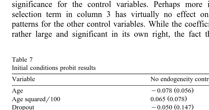
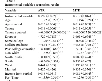
Mills ratio from the first-stage probit of the initial condition Tables 7 and 8 present results from first-stage selection and instrumenting regressions. Also, Table 9 contains results from a baseline probit without random effects. Note that magnitudes of the coefficients and patterns of significance are essentially

un-. changed in the absence of the random effects .

Comparing the first two columns shows that the different sample required for the initial conditions correction results in only minor differences in patterns of significance for the control variables. Perhaps more importantly, adding the selection term in column 3 has virtually no effect on signs and significance patterns for the other control variables. While the coefficient on the Mills ratio is rather large and significant in its own right, the fact that its inclusion has no

Table 7

Income from capital y0.021 0.011

Ž .

Part-time y0.040 0.110

Ž .

Number of children 0.041 0.050

N 1391

Entries are probit coefficients with standard errors in parentheses. This regression also includes indicators for the year of the observation and a constant term. The dependent variable is a dummy which equals 1 for wage-and-salary employment in the first observed job, and zero for self-employed.

(19)

Table 8

Instrumental variables regression results

Variable ATR MTR Income

) ) ) )

Ž . Ž . Ž .

Instrumental variable 0.897 0.087 0.519 0.016 0.15 0.19

) ) ) )

Ž . Ž . Ž .

Age y1.223 0.273 y1.196 0.241 y223.57 262.72

) ) ) )

Ž . Ž . Ž .

Age squared 0.015 0.004 0.014 0.003 y0.94 3.75

) ) ) ) ) )

Ž . Ž . Ž .

Tenure 0.019 0.006 0.011 0.005 18.11 5.54

) ) ) )

Ž . Ž . Ž .

Tenure squared y0.00007 0.00003 y0.00007 0.00002 y0.03 0.02

) ) ) ) ) )

Ž . Ž . Ž .

Dropout 4.727 0.718 3.665 0.674 2416.26 810.86

) ) ) ) )

Ž . Ž . Ž .

Some college y1.904 0.511 y0.808 0.482 y1536.39 582.76

) ) ) ) ) )

Ž . Ž . Ž .

College graduate y4.647 0.575 y5.815 0.552 y7617.04 654.70

) ) ) ) ) )

Ž . Ž . Ž .

Post-college education y6.180 0.662 y5.041 0.648 y14,653.62 749.76

) ) ) ) ) )

Ž . Ž . Ž .

Non-white y1.625 0.692 y1.727 0.642 y3167.84 754.57

)

Ž . Ž . Ž .

North Central y0.102 0.532 0.889 0.494 445.02 580.31

) )

Ž . Ž . Ž .

South y0.769 0.507 0.353 0.467 y1789.82 540.57

) )

Ž . Ž . Ž .

West 0.441 0.563 1.193 0.521 y107.02 608.43

) ) ) )

Ž . Ž . Ž .

Married 0.425 0.426 0.833 0.370 918.17 394.21

) ) )

Ž . Ž . Ž .

Income from capital 0.018 0.051 0.086 0.044 131.16 46.02

) ) ) ) ) )

Ž . Ž . Ž .

Part-Time y1.356 0.366 y1.296 0.310 y1114.90 323.89

) ) )

Ž . Ž . Ž .

Kids 1 to 2 0.442 0.242 0.123 0.206 634.92 214.00

)

Ž . Ž . Ž .

Kids 3 to 5 0.390 0.248 0.224 0.212 403.88 221.83

Ž . Ž . Ž .

Kids 6 to 13 y0.053 0.218 0.153 0.191 y50.43 207.51

Ž . Ž . Ž .

Kids 14 to 17 y0.041 0.439 y0.596 0.375 y210.50 393.76

) )

Ž . Ž . Ž .

Union 1.147 0.402 0.546 0.353 608.31 381.07

) ) )

Ž . Ž . Ž .

Unemployment rate y0.114 0.059 y0.051 0.051 y240.23 54.60

Ž . Ž . Ž .

MSA 0.399 0.342 0.436 0.304 518.63 336.21

N 5622 5622 5515

2_Ž _.

R overall 0.17 0.24 0.29

Entries are GLS random-effects regression coefficients with standard errors in parentheses. Regressions also include indicators for the year of the observation and a constant term.

)_{Statistically significant at the 10% level.} ) )_{Statistically significant at the 5% level.}

discernible effect on the other coefficients should be somewhat reassuring to those researchers who have not performed this correction in previous work. The statistical significance indicates that initial conditions clearly matter in the self-em-ployment transition process, however, so all remaining probits will include a selection term.

Before moving to the analysis of tax effects, note that the effects of the other variables in column 3 are generally consistent with findings in earlier studies. First, age affects the transition probability in a u-shaped manner in the corrected specification. Those at the younger and older extremes of the age distribution are more likely to enter. Tenure on the wage-and-salary job also affects this probabil-ity in a u-shaped manner. Essentially, those who enter self-employment are likely to have spent either a very little or a very long time in their pre-transition job.

Minorities and union members are significantly less likely to enter

self-employ-Ž .

(20)

564 Table 9

Self-employment transition probit without random effects

Variable No endogeneity control

Income from capital 0.004 0.002

) )

Kids 14 to 17 y0.001 0.038

) )

Entries are probit coefficients with standard errors in parentheses. This regression also includes indicators for the year of the observation and a constant term. For comparison purposes, the sample for

Ž .

this probit is identical to that in column 1 of Table 6 which includes random effects .

Ž .

among others, and is explained by Blanchflower et al. 1998 as the result of racial discrimination in lending markets. The union membership indicator is likely capturing an important job-lock effect. The effect of children in the household depends on their age distribution. Having more children in the household between the ages of 3 and 5 increases the transition probability, while having more children who are between the ages of 14 and 17 reduces the probability. This is presumably a result of the fact that the younger children can be placed in daycare or nursery school facilities, and the older children might be preparing to enter college. A parent’s attitude toward the inherent risk of becoming self-employed might carry different weights at these times.

While not the primary focus of this study, it is important to address the effect of unemployment on self-employment. Indeed, this relationship has received a great deal of attention in recent research and no significant degree of consensus has

Ž .

(21)

rates have a negative impact on self-employment transitions. This divergence is likely due to different degrees of aggregation in the respective unemployment rate variables. Schuetze used state-level unemployment rates, while I use county-level unemployment rates. Higher unemployment at the local level might reduce one’s probability of becoming self-employed by reducing the likelihood that he would be able to regain wage-and-salary employment should his business fail. State unemployment rates, however, more closely reflect macroeconomic effects such as the degree of downsizing in the economy. In this way, higher unemployment on an aggregate level indicates that workers might be turned toward self-employment as a result of actually losing their wage-and-salary jobs.

Turning now to Table 10, the effect of controlling for differential tax treatment on the self-employment entry decision is observed. This table presents results from

Table 10

Pooled transition probit results: using marginal tax rate differentials

Variable No endogeneity control IV for MTR differential

) )

Ž . Ž .

Age y0.079 0.052 y0.275 0.063

) )

Ž . Ž .

Age squaredr100 0.109 0.077 0.353 0.093

) ) ) )

Ž . Ž .

Tenure y0.006 0.001 y0.004 0.002

) )

Ž . Ž .

Tenure squaredr100 0.100 0.047 y0.011 0.066

) )

Ž . Ž .

Dropout y0.014 0.142 0.508 0.157

Ž . Ž .

Some college y0.011 0.097 y0.051 0.113

) )

Ž . Ž .

College graduate 0.046 0.106 y0.363 0.116

Ž . Ž .

Post-college education 0.126 0.106 0.007 0.121

) ) ) )

Ž . Ž .

Non-white y0.279 0.142 y0.449 0.149

Ž . Ž .

North Central y0.037 0.103 0.061 0.120

Ž . Ž .

South y0.108 0.097 y0.081 0.124

Ž . Ž .

West 0.048 0.097 0.195 0.123

Ž . Ž .

Married 0.090 0.095 0.160 0.115

Ž . Ž .

Income from capital y0.013 0.012 0.008 0.014

)

Ž . Ž .

Part-time 0.158 0.085 y0.007 0.107

Ž . Ž .

Kids 1 to 2 y0.044 0.063 y0.005 0.070

) ) ) )

Ž . Ž .

Kids 3 to 5 0.250 0.061 0.286 0.066

Ž . Ž .

Kids 6 to 13 0.055 0.055 0.060 0.058

) ) )

Ž . Ž .

Kids 14 to 17 y0.240 0.111 y0.263 0.145

) ) ) )

Ž . Ž .

Union y0.407 0.115 y0.309 0.126

) ) ) )

Ž . Ž .

Unemployment rate y0.045 0.012 y0.055 0.014

Ž . Ž .

MSA 0.003 0.079 0.060 0.085

) ) )

Ž . Ž .

Mills ratio 0.954 0.502 1.173 0.538

) ) ) )

Ž . Ž .

MTR differential 0.017 0.004 y0.123 0.010

N 5622 5622

Sample transition probability 0.033 0.033

Entries are random-effects probit coefficients with bootstrapped robust standard errors in parentheses. Regressions also include indicators for the year of the observation and a constant term. The first-stage instrumenting equation includes an identical set of variables in addition to the instrument.

(22)

566

Ž

random effects transition probits that include the wage-and-salary minus

self-em-. Ž .

ployment difference in marginal tax rates MTR . The first column contains coefficients and bootstrapped standard errors without instrumenting for the tax rate differential.12 Column 1 shows that the MTR differential has a very small positive and significant effect on the probability of entry. This indicates that those with a larger last-dollar tax benefit from entering self-employment are also more likely to be the ones who choose to enter.

The question of endogeneity remains, however, so column 2 presents results from a two-stage instrumental variables estimation process as described above. While patterns of significance for the non-tax variables remain largely unchanged, the effect of the instrumented tax rate differential is now negative, much larger, and even more statistically significant. To determine the extent to which endogene-ity is an actual problem in this situation, I performed the test suggested by Rivers

Ž .

and Vuong 1988 . This test involves inserting the potentially endogenous variable along with the estimated residual vector from the proposed first-stage instrument-ing equation into the transition probit. A significant coefficient on the residual indicates that endogeneity is a serious problem. Indeed, the Rivers–Vuong test for this random effects probit rejects the null hypothesis of exogeneity — the coefficient on the residual term is statistically significant.

A simulation is helpful in understanding the quantitative significance of the instrumented MTR differential in column 2. Increasing this differential by 5 percentage points causes a reduction in the average self-employment transition probability of about 2.4 percentage points. This yields an elasticity of

approxi-matelyy0.60.

Table 11 is similar to Table 10, except that it uses a difference in average tax

Ž . Ž .

rates ATR . As with the MTR differential without instrumenting , the effect of the ATR differential is small but positive and statistically significant. Column 2 presents results from a similar two-stage instrumental variables estimation process in order to investigate the potential endogeneity of the ATR differential. Again, patterns of significance for the non-tax variables remain largely unchanged. However, the effect of the instrumented tax rate differential is now negative, as with the MTR differential, but not statistically significant. In this case, though, the Rivers–Vuong test fails to reject the null hypothesis of exogeneity.

Using the results in column 1, then, increasing the ATR differential by 5 percentage points would increase the average self-employment transition probabil-ity by only about 0.4 percentage points. This effect is especially small in

12

(23)

Table 11

Pooled transition probit results: using average tax rate differentials

Variable No Endogeneity Control IV for ATR Differential

Ž . Ž .

Age y0.082 0.052 y0.099 0.079

Ž . Ž .

Age squaredr100 0.112 0.077 0.132 0.117

) ) ) )

Ž . Ž .

Tenure y0.006 0.001 y0.005 0.002

) )

Ž . Ž .

Tenure squaredr100 0.094 0.045 0.080 0.081

Ž . Ž .

Dropout y0.012 0.132 0.061 0.185

Ž . Ž .

Some college 0.005 0.095 y0.025 0.106

Ž . Ž .

) )

Ž . Ž .

Non-white y0.283 0.142 y0.293 0.182

Ž . Ž .

North Central y0.030 0.105 y0.031 0.100

Ž . Ž .

South y0.105 0.099 y0.111 0.086

Ž . Ž .

West 0.059 0.097 0.070 0.106

Ž . Ž .

Married 0.101 0.095 0.103 0.084

Ž . Ž .

Income from capital y0.012 0.012 y0.011 0.017

Ž . Ž .

Part-time 0.159 0.085 0.131 0.083

Ž . Ž .

Kids 1 to 2 y0.051 0.064 y0.046 0.059

) ) ) )

Ž . Ž .

Kids 3 to 5 0.243 0.060 0.246 0.067

Ž . Ž .

Kids 6 to 13 0.051 0.055 0.050 0.052

)

Ž . Ž .

Kids 14 to 17 y0.215 0.115 y0.206 0.174

) ) ) )

Ž . Ž .

Union y0.400 0.109 y0.376 0.117

) ) ) )

Ž . Ž .

MSA 0.013 0.077 0.018 0.076

) ) ) )

Ž . Ž .

Mills ratio 0.994 0.504 0.956 0.417

) )

Ž . Ž .

ATR differential 0.010 0.003 y0.006 0.031

N 5622 5622

Entries are random-effects probit coefficients with bootstrapped robust standard errors in parentheses. Regressions also include indicators for the year of the observation and a constant term. The first-stage instrumenting equation includes an identical set of variables in addition to the instrument.

comparison to the sample transition probability of 3.3%, translating into an elasticity of about 0.06.

Table 12 examines whether ATRs and MTRs truly have these opposing effects by including both variables in a single random effects probit. Column 1 contains results without instrumental variables, while column 2 presents the IV results. The results in Tables 10 and 11 are seen again in this specification and, in fact, are essentially unchanged. Those contemplating a transition into self-employment are apparently more responsive to changes at the margin than they are to changes in average tax rates. The Rivers–Vuong test rejects the null hypothesis of joint exogeneity in this case.

(24)

568 Table 12

Pooled transition probit results: using average and marginal tax rate differentials

Variable No endogeneity control IV for ATR and MTR differentials

) )

Ž . Ž .

Age y0.075 0.052 y0.268 0.075

) )

Ž . Ž .

Age squaredr100 0.104 0.078 0.344 0.108

) ) ) )

Ž . Ž .

Tenure y0.006 0.001 y0.004 0.002

) )

Ž . Ž .

) )

Ž . Ž .

Dropout y0.038 0.146 0.481 0.200

Ž . Ž .

Some college y0.001 0.096 y0.040 0.125

) )

Ž . Ž .

) ) ) )

Ž . Ž .

Non-white y0.282 0.143 y0.439 0.152

Ž . Ž .

North Central y0.036 0.104 0.062 0.120

Ž . Ž .

South y0.107 0.098 y0.076 0.124

Ž . Ž .

West 0.045 0.098 0.192 0.128

Ž . Ž .

Married 0.093 0.095 0.157 0.118

Ž . Ž .

) )

Ž . Ž .

Part-time 0.167 0.085 0.002 0.115

Ž . Ž .

Kids 1 to 2 y0.047 0.063 y0.008 0.071

) ) ) )

Ž . Ž .

Kids 3 to 5 0.249 0.061 0.284 0.065

Ž . Ž .

Kids 6 to 13 0.055 0.056 0.060 0.059

) ) )

Ž . Ž .

Kids 14 to 17 y0.242 0.112 y0.263 0.148

) ) ) )

Ž . Ž .

Union y0.415 0.115 y0.315 0.131

) ) ) )

Ž . Ž .

MSA 0.003 0.079 0.059 0.080

) ) )

Ž . Ž .

Mills ratio 0.975 0.502 1.175 0.540

) )

Ž . Ž .

ATR differential 0.006 0.003 0.006 0.026

) ) ) )

Ž . Ž .

N 5622 5622

Entries are random-effects probit coefficients with bootstrapped robust standard errors in parentheses. Regressions also include indicators for the year of the observation and a constant term. The first-stage instrumenting equations include an identical set of variables in addition to the instruments.

those with the largest tax advantage per dollar of income are slightly more likely to enter self-employment, although the quantitative effect is small. However, the statistically and quantitatively more significant negative impact of the instru-mented MTR differential reveals an opposite effect.

(25)

The extent to which this is an income effect rather than a price effect can be examined by including the difference in after-tax household income as a regressor in addition to the MTR differential. Table 13 presents results from two probits,

Ž . Ž .

without column 1 and with column 2 similar instrumenting equations for the MTR and net income differentials. In column 1, the MTR effect is apparently unchanged but the coefficient on the net income differential is strangely positive Žand significant , indicating that larger expected income reductions from entering. self-employment actually increase the probability of entry.

However, the results in column 2 show that instrumenting for both of the potentially endogenous differential variables renders the income effect statistically insignificant. In fact, the only variables with any significance are the Mills ratio for the initial conditions correction and the MTR differential. The Rivers–Vuong

Table 13

Pooled transition probit results: adding after-tax household income differentials

Variable No endogeneity control IV for after-tax difference

Ž . Ž .

Age y0.091 0.056 y0.357 0.654

Ž . Ž .

Age squaredr100 0.130 0.082 0.352 0.618

) )

Ž . Ž .

Tenure y0.006 0.002 0.001 0.020

Ž . Ž .

Dropout y0.046 0.150 1.199 2.567

Ž . Ž .

Some college 0.026 0.085 y0.477 1.453

Ž . Ž .

) )

Ž . Ž .

Post-college education 0.297 0.115 y4.216 13.786

Ž . Ž .

Non-white y0.222 0.163 y1.342 2.744

Ž . Ž .

North Central y0.070 0.096 0.174 0.936

Ž . Ž .

South y0.107 0.075 y0.601 1.376

Ž . Ž .

West 0.047 0.076 0.179 0.519

Ž . Ž .

Married 0.084 0.099 0.428 1.157

Ž . Ž .

) )

Ž . Ž .

Part-time 0.213 0.084 y0.327 0.966

Ž . Ž .

Kids 1 to 2 y0.038 0.054 0.196 0.513

) )

Ž . Ž .

Kids 3 to 5 0.224 0.062 0.386 0.477

Ž . Ž .

Kids 6 to 13 0.056 0.062 0.042 0.338

Ž . Ž .

Kids 14 to 17 y0.208 0.151 y0.304 0.430

) )

Ž . Ž .

Union y0.449 0.126 y0.166 0.472

) )

Ž . Ž .

MSA y7.69ey05 0.063 0.229 0.305

) ) ) )

Ž . Ž .

Mills ratio 1.015 0.407 1.068 0.368

) ) ) )

Ž . Ž .

) )

Ž . Ž .

Income differential 1.95ey05 3.48ey06 y2.86ey04 9.75ey04

N 5515 5515

Entries are random-effects probit coefficients with bootstrapped robust standard errors in parentheses. Regressions also include indicators for the year of the observation and a constant term. The first-stage instrumenting equations include an identical set of variables in addition to the instruments.

(26)

570

test rejects the null hypothesis of joint exogeneity, and the effect of the instru-mented MTR differential itself is unchanged.

6. Conclusions

Workers considering a switch to self-employment are apparently aware of their individual-level tax situations. This paper has shown that the differential tax treatment of wage-and-salary and self-employment income has important effects on transition probabilities. Specifically, larger individual-specific differences in marginal tax rates in the two sectors are found to reduce self-employment entry rates. This effect is independent of the difference in after-tax incomes. Individual average tax rate differentials have much smaller positive effects. Finally, control-ling for initial-conditions bias is found to be important, despite the fact that the overall empirical findings seem to be unaffected.

These results are somewhat consistent with the conclusion in earlier studies that higher marginal tax rates increase self-employment. However, the reasoning behind this effect is not one of potential entrepreneurs simply escaping higher wage-and-salary taxes. If this were the case, as noted above, the sign on the MTR differential would be positive. Instead, this study has found that those who would

Ž .

have higher marginal tax rates in self-employment and lower MTR differentials are more likely to become self-employed.

An important effect that has been mentioned but not directly addressed in this paper is that of tax avoidance or evasion. Specifically, a higher marginal tax rate in self-employment increases the tax benefit for a given level of business-related deductions, and increases the reward to reducing taxable income in other legal or illegal ways. My results could be interpreted as evidence that those who stand to gain the most in these ways are more likely to enter self-employment. Certainly, more research is warranted.

Further, little is known about the presence of tax effects on those who are

Ž .

already self-employed. The differential tax treatment and increased complexity might also hasten the departure of marginally successful entrepreneurs, thereby compounding the entry effects found in this paper. A dynamic analysis of self-employment duration would be useful in examining this possibility.

Acknowledgements

(27)

Office of Tax Policy Research at the University of Michigan for providing access to and assistance with the Ernst and Young Tax Research Database; Barbara Butrica and Don Marples in the Center for Policy Research at Syracuse University for assistance with the PSID; Becky Porcello for outstanding research assistance; and Jim Bruce, Jamie Emerson, Susan Gensemer, Peter Kuhn, Alan Macnaughton, Raymond Robertson, Harvey Rosen, Katherin Ross, Herb Schuetze, Bob Weath-ers, one anonymous referee and seminar participants at Syracuse University, the University of Tennessee, Transylvania University, and St. Lawrence University for helpful comments. Full responsibility for any remaining errors is mine alone.

Appendix A. Note on the calculation of tax rates for the PSID using the National Bureau of Economic Research TAXSIM Model

The income tax rates used in this paper were all calculated using the National

Ž .

Bureau of Economic Research NBER TAXSIM model. While the Panel Study of

Ž .

Income Dynamics PSID contains assorted federal tax variables, the use of

TAXSIM enables the consistent calculation of a richer set of tax information for various individual characteristics. Further, it allows the calculation of both federal and state taxes. For more specific information regarding TAXSIM, see

Ž .

Feenberg and Coutts 1993 or the internet version of TAXSIM, available at http:rrwww.nber.orgr;taxsimrtaxsim.html.

In calculating the baseline, or actual income tax rates for this paper, I followed

Ž .

the method of Butrica and Burkhauser 1997 with two exceptions. First, out of convenience, they combined the labor income of the head and spouse into one variable. I separated these in order to more easily analyze changes in the head’s labor income. Second, they assumed that all filers took the standard deduction for their calculations, while I make use of a rich set of tax return data to impute itemized deductions. All other variables are created exactly as in Butrica and

Ž .

Burkhauser 1997 . Specifically, TAXSIM requires information on tax filing

status, state of residence, the number of dependent exemptions, the number of old age exemptions, taxable income in various categories, and expenditures on rent, property taxes, and child care. Since their purpose was to provide alternative tax

Ž .

variables to those provided in the PSID, Butrica and Burkhauser 1997 follow PSID conventions whenever possible in creating their TAXSIM input variables.

Ž .

The major deviation from Butrica and Burkhauser 1997 in this paper is the imputation of itemized deductions. Respondents in the PSID do not report the dollar value of total deductions. In fact, this variable is estimated in the calculation

Ž

of the PSID tax data. Specifically, the PSID predicts or, from 1984 on, actually .

asks whether or not a tax unit itemized deductions in the previous year. Those predicted or observed to have itemized are assigned weighted-average deduction

Ž .

amounts for their income bracket, based on IRS Statistics of Income SOI reports.

Ž .