Conference paper

BUNDLE ADJUSTMENT FOR MULTI-CAMERA SYSTEMS WITH POINTS AT INFINITY

Johannes Schneider, Falko Schindler, Thomas L¨abe, Wolfgang F¨orstner

University Bonn, Institute for Geodesy and Geoinformation Department of Photogrammetry, Nussallee 15, 53115 Bonn, Germany

[johannes.schneider|falko.schindler]@uni-bonn.de,[laebe|wf]@ipb.uni-bonn.de, http://www.ipb.uni-bonn.de

KEY WORDS:bundle adjustment, omnidirectional cameras, multisensor camera, ideal points, orientation

ABSTRACT:

We present a novel approach for a rigorous bundle adjustment for omnidirectional and multi-view cameras, which enables an efficient maximum-likelihood estimation with image and scene points at infinity. Multi-camera systems are used to increase the resolution, to combine cameras with different spectral sensitivities (Z/I DMC, Vexcel Ultracam) or – like omnidirectional cameras – to augment the effective aperture angle (Blom Pictometry, Rollei Panoscan Mark III). Additionally multi-camera systems gain in importance for the acquisition of complex 3D structures. For stabilizing camera orientations – especially rotations – one should generally use points at the horizon over long periods of time within the bundle adjustment that classical bundle adjustment programs are not capable of. We use a minimal representation of homogeneous coordinates for image and scene points. Instead of eliminating the scale factor of the homogeneous vectors by Euclidean normalization, we normalize the homogeneous coordinates spherically. This way we can use images of omnidirectional cameras with single-view point like fisheye cameras and scene points, which are far away or at infinity. We demonstrate the feasibility and the potential of our approach on real data taken with a single camera, the stereo cameraFinePix Real 3D W3from Fujifilm and the multi-camera systemLadybug 3from Point Grey.

1 INTRODUCTION

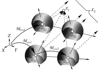
Motivation. The paper presents a novel approach for the bundle adjustment for omnidirectional and multi-view cameras, which enables the use of image and scene points at infinity, called “BACS” (Bundle Adjustment for Camera Systems). Bundle ad-justmentis the work horse for orienting cameras and determining 3D points. It has a number of favourable properties: It is sta-tistically optimal in case all statistical tools are exploited, highly efficient in case sparse matrix operations are used, useful for test field free self calibration and can be parallelized to a high degree. Multi-camera systemsare used to increase the resolution, to com-bine cameras with different spectral sensitivities (Z/I DMC, Vex-cel Ultracam) or – likeomnidirectional cameras– to augment the effective aperture angle (Blom Pictometry, Rollei Panoscan Mark III). Additionally multi-camera systems gain importance for the acquisition of complex 3D structures. Far or even ideal points, i. e. points at infinity, e. g. points at the horizon are effective in stabilizing the orientation of cameras, especially their rotation. In order to exploit the power of bundle adjustment, it therefore needs to be extended to handle multi-camera systems and image and scene points at infinity, see Fig. 1.

The idea. The classical collinearity equations for image points

x

′

it([x ′ it;y

′

it]) of scene point

Xi

([Xi;Yi;Zi]) in cameratwith rotation matrix

Rt

([rkk′])withkandk

′

= 1, ...,3and projection center

Zt

([X0t;Y0t;Z0t])read as

x′ it=

r11(Xi−X0t) +r21(Yi−Y0t) +r31(Zi−Z0t)

r13(Xi−X0t) +r23(Yi−Y0t) +r33(Zi−Z0t) (1)

y′ it=

r12(Xi−X0t) +r22(Yi−Y0t) +r32(Zi−Z0t)

r13(Xi−X0t) +r23(Yi−Y0t) +r33(Zi−Z0t) (2)

Obviously, these equations are not useful for far points or ideal points, as small angles between rays lead to numerical instabil-ities or singularinstabil-ities. They are not useful for bundles of rays of omnidirectional cameras, as rays perpendicular to the view-ing direction, as they may occur with fisheye cameras, cannot be transformed into image coordinates. This would require differ-ent versions of the collinearity equation depending on the type

Figure 1: A two-camera system with Fisheye camerasc= 1,2 with projection centers

Ztc

and known motion

Mc

and unknown motion

Mt

, having a field of view larger than180◦

shown at two exposure timest= 1,2observing two points

Xi

, i= 1,2, one being close, the other at infinity. Already a block adjustment with a single camera moving over time will be stabilized by points at infinity.

of sensor as one would need to integrate the camera model into the bundle adjustment. Finally, the equations are not easily ex-tensible to systems of multiple cameras, as one would need to integrate an additional motion, namely, the motion from the co-ordinate system of the camera system to the individual camera systems, which appears to make the equations explode.

Geometrically this could be solved by using homogeneous coor-dinatesx′

itandXifor image and scene points, a calibration ma-trixKtand the motion matrixMtin:x′

it=λit[Kt|0]M −1

t Xi=

λitPtXi. Obviously, (a) homogeneous image coordinates allow for ideal image points, even directions opposite to the viewing direction, (b) homogeneous scene coordinates allow for far and ideal scene points, and including an additional motion is simply an additional factor.

However, this leads to two problems. As the covariance matri-cesΣx′

λitPtXi|

2

Σ−x′1

itxit′

is not valid. A minor, but practical problem is the

increase of the number of unknown parameters, namely the La-grangian multipliers, which are necessary when fixing the length of the vectorsXi. In large bundle adjustments with more than a million scene points this prohibitively increases the number of unknowns by a factor 5/3.

Task and challenges. The task is to model the projection pro-cess of a camera system as the basis for a bundle adjustment for a multi-view camera system, which consists of mutually fixed single view cameras, which allows the single cameras to be om-nidirectional, requiring to explicitly model the camera rays and which allows for far or ideal scene points for stabilizing the con-figuration. The model formally reads as

xitc

=

Ptc

(

M

−1

t (

Xi

)) (3)

with theI scene points

Xi

, i= 1, ..., I, theT motions

Mt

, t= 1, ..., Tof the camera systems from origin, the projection

Ptc

into the camerasc= 1, ..., Cpossibly varying over time, and the ob-served image points

xitc

of scene pointiin cameracat time/poset.

For realizing this we need to be able to represent bundles of rays together with their uncertainty, using uncertain direction vectors, to represent scene points at infinity using homogeneous coordi-nates, and minimize the number of parameters to be estimated. The main challenge lies in the inclusion of the statistics into an adequate minimal representation.

Related Work. Multi-camera systems are proposed by many authors. E. g. Mostafa and Schwarz (2001) present an approach to integrate a multi-camera system with GPS and INS. Nister et al. (2004) discuss the advantage to use a stereo video rig in or-der to avoid the difficulty with the scale transfer. Savopol et al. (2000) report on a multi-camera system for an aerial platform for increasing the resolution. In all cases the multi view geometry is only used locally. Orientationof a stereo rig is discussed in Hartley and Zisserman (2000, p. 493). Mouragnon et al. (2009) proposed a bundle solution for stereo rigs working in terms of di-rection vectors, but they minimize the angular error without con-sidering the covariance matrix of the observed rays. Frahm et al. (2004) present an approach for orienting a multi-camera system, however not applying a statistically rigorous approach. Muhle et al. (2011) discuss the ability to calibrate a multi-camera system in case the views of the individual cameras are not overlapping. Zomet et al. (2001) discuss the problem of re-calibrating a rig of cameras due to changes of the internal parameters. Bundle adjust-ment of camera systems have been extensively discussed in the thesis of Kim (2010).Uncertain geometric reasoningusing pro-jective entities has extensively been presented in Kanatani (1996), but only using Euclideanly normalized geometric entities and re-stricting estimation to single geometric entities. Heuel (2004) eliminating these deficiencies, proposed an estimation procedure which does not eliminate the redundancy of the representation and also cannot easily include elementary constraints between observations, see Meidow et al. (2009). The following develop-ments are based on the minimal representation schemes proposed in F¨orstner (2012) which reviews previous work and generalizes e. g. Bartoli (2002).

2 CONCEPT

2.1 Model for sets of single cameras

2.1.1 Image coordinates as observations. Using homoge-neous coordinates

x′

it=λitPtXi=λitKtRTt[I3| −Zt]Xi (4) with a projection matrix

Pt= [Kt|03×1]M

−1

t , Mt= _R

t Zt 0T 1

(5)

makes the motion of the camera explicit. It contains for each pose

t: the projection centerZtin scene coordinate system, i. e. trans-lation of scene system to camera system, the rotation matrixR_t

of scene system to camera system, and the calibration matrix_Kt, containing parameters for the principal point, the principal dis-tance, the affinity, and possibly lens distortion, see McGlone et al. (2004, eq. (3.149) ff.) and eq. (12). In case of an ideal camera with principal distancecthus_Kt=Diag([c, c,1])and Euclidean normalization of the homogeneous image coordinates with the

k-th rowAT_t,kof the projection matrixPt

x′e it = P

tXi AT

t,3Xi =

 

AT_t,1Xi/ATt,3Xi AT

t,2Xi/ATt,3Xi 1



 (6)

we obtain eq. (1), e. g.x′

it=ATt,1Xi/ATt,3Xi.

Observe the transposition of the rotation matrix in eq. (4), which differs from Hartley and Zisserman (2000, eq. (6.7)), but makes the motion of the camera from the origin into the actual camera system explicit, see Kraus (1997).

2.1.2 Ray directions as observations. Using the directions from the cameras to the scene points we obtain the collinearity equations

k_x′

it=λitkPtXi=λitRTt(Xi−Zt) =λit[I3 |0]M

−1

t Xi. (7) Instead of Euclidean normalization, we now perform spherical normalizationxs ₌

N(x_{) =} x_/|x_{|yielding the collinearity} equations for camera bundles

k_x′s

it=N(kPtXi). (8)

We thus assume the camera bundles to be given as T sets {k_x

it, i∈ It}of normalized directions for each timetof expo-sure. The unknown parameters are the six parameters of the mo-tion ink_Ptand the three parameters of each scene point. Care has to be taken with the sign: We assume the negativeZ-coordinate of the camera system to be the viewing direction. The scene points then need to have non-negative homogeneous coordinate

Xi,4, which in case they are derived from Euclidean coordinates

viaX_{i = [Xi; 1]always is fulfilled. In case of ideal points, we} therefore need to distinguish the scene point[Xi; 0]and the scene point[−Xi; 0]which are points at infinity in opposite directions. As a first result we observe: The difference between the classical collinearity equations and the collinearity equations for camera bundles is twofold. (1) The unknown scale factor is eliminated differently: Euclidean normalization leads to the classical form in eq. (6), spherical normalization leads to the bundle form in eq. (8). (2) The calibration is handled differently: In the classi-cal form it is made explicit, here we assume the image data to be transformed into camera rays taking the calibration into account. This will make a difference in modelling the camera during self-calibration, a topic we will not discuss in this paper.

normalized coordinates for the scene points leading to

k_x′s

it=N(kPtXsi). (9)

Again care has to be taken with points at infinity.

2.2 Model for sets of camera systems

With an additional motion_Mc(Rc,Zc)for each camera of the camera system we obtain the general model for camera bundles

k_x′s

making all elements explicit: the calibration of the camera system (Mc, c= 1, . . . , C), assumed to be rigid over time, and the pose

with observed directions

x

′ itc(kx

′

itc)represented by normalized 3-vectors, having two degrees of freedom, unknown or known scene point coordinates

Xi

(Xs_i), represented by spherically nor-malized homogeneous 4-vectors, having 3 degrees of freedom and unknown pose

Mt

of camera system, thus 6 parameters per time. The projection matriceskPconly containing the relative pose of the camerasMcare assumed to be given in the following.

2.3 Generating camera directions from observed image co-ordinates

In most cases the observations are made using digital cameras which physically are – approximately – planar. The transition to directions of camera rays need to be performed before starting the bundle adjustment. As mentioned before, this requires the internal camera geometry to be known. Moreover, in order to arrive at a statistically optimal solution, one needs to transfer the uncertainty of the observed image coordinates to the uncertainty of the camera rays. As an example we discuss two cases.

Perspective cameras. In case we have perspective cameras with small image distortions, we can use the camera-specific and maybe temporal varying calibration matrix

K(x′,q) =

from the observed image coordinatesg_x′

, theg _{indicating the} generality of the mapping system and the ray directions kx′s. The calibration matrix besides the basic parameters, namely the principal distancecwith image planek_{Z =c, shears, scale} dif-ferencem, and principal pointx′

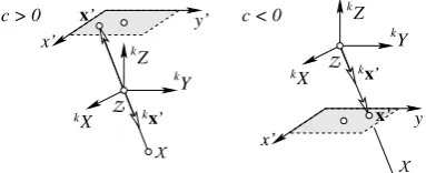
H, contains additive corrections for modelling lens distortion or other deviations, which depend on additional parametersq and are spatially different viax. In case of small deviations eq. (13) can easily be inverted. However, one must take into account, the different sign of the coordinate vector and the direction from the camera to the scene point, see Fig. 2,

k

x′s≈sN K−1

(gx′,q)gx′ (14)

withs ∈ {−1,+1}such thatkx′s3 < 0. This relation is

inde-pendent of the sign of the third element of the calibration matrix.

x’

Figure 2: The direction of the homogeneous image coordinate vector and the direction of the ray is different depending on the sign of the principal distancec.

Given the covariance matrixΣgx′x′of the image coordinates, the

covariance matrix ofkx′ can be determined by variance propa-gation, omitting the dependency of the calibration matrix on the point coordinatesx′

. Note that a pointg_x′

at infinity corresponds to the directionkx′perpendicular to the viewing direction.

Omnidirectional single view point cameras. As an example for an omnidirectional single view camera we take a camera with a fisheye-lens. In the most simple case the normalized radial dis-tancer′

= px′2_+y′2_{/cof an image point with coordinates}

[x′

, y′

]being the reduced image coordinates referring to the prin-cipal point, goes with the angleφbetween the viewing direction and the camera ray. A classical model is the stereographic model

r′

Again, the uncertainty of the image coordinates can be trans-formed to the uncertainty of the directionkx′s_{of the camera ray} via variance propagation. In all cases the covariance matrix of the camera rays is singular, as the normalized 3-vector only depends on two observed image coordinates.

2.4 The estimation procedure

The collinearity equations in (11) contain three equations per observed camera ray and four parameters for the scene points, though, both being unit vectors. Therefore the corresponding co-variance matrices are singular and more than the necessary pa-rameters are contained in the equations. We therefore want to reduce the number of parameters to the necessary minimum. We do this after linearization.

Linearization and update for pose parameters. Linearization of the non-linear model leads to a linear substitute model which yields correction parameters which allow to derive corrected ap-proximate values. We start with apap-proximate valuesRa

for the rotation matrix,Za_{for the projection center,X}sa_{for the} spher-ically normalized scene points, andxa = N(P (Ma₎−1

Xa) for the normalized directions. The Euclidean coordinates will be simply corrected byZ =Za_{+ ∆Z, the three parameters∆Z} are to be estimated. The rotation matrix will be corrected by pre-multiplication of a small rotation, thus byR ₌ R_(∆R)Ra _≈ (I3+S(∆R))Ra, where the small rotationR(∆R)depends on

a small rotation vector∆Rthat is to be estimated.

Reduced coordinates and update of coordinates. The correc-tion of the unit vectors is performed using reduced coordinates. These are coordinates, say the two-vectorxrof the directionxs, in the two-dimensional tangent space null xsaT_{= [r,s]of the} unit sphereS2

evaluated at the approximate valuesxsa

The corrections∆xrof these reduced coordinates are estimated. This leads to the following update rule

xs=Nxsa+nullxsaT∆xr. (16)

Obviously, the approximate vectorxsais corrected by

∆x_=nullxsaT_{∆xr (17)}

and then spherically normalized to achieve the updated values xs. Using (15) we now are able to reduce the number of equa-tions per direction from three to two, making the degrees of free-dom of the observed direction, being two, explicit. This results in pre-multiplication of all observation equations on (11) with nullTkxsa_itcT. When linearizing the scene coordinates we, fol-lowing (17), use the substitution∆Xs_i = null Xsa_i T∆Xr,i. Then we obtain the linearized model

k

xr,itc+_bvxr,itc (18)

= −kJT_skxa_itc R_tcaTS₍Xai0)∆dRt

+kJT_skxa_itc Ra_tcT_Xiha_∆d_{Zt (19)}

+kJT_skx_itca k_Pc(Mat) −1

nullXa_iT∆dXri

with

k_J s(kx

a itc) =

1 |x_|

I3−

xxT

xTx

null(xT_{) x=}k

xa_itc (20)

partitioning of the homogeneous vectorXs= [X0;Xh]and the compound rotation matrixRa

tc=R a

tRcdepending on∆dR,∆dZ, and\∆Xr.

We now arrive at a well defined optimization problem: find d

∆Xr,i,∆dRt,∆dZtminimizing

Ω∆dXr,i,∆dRt,∆dZt=X itc

b

vTr,itcΣ−xr,itcxr,itc1 vr,itcb (21)

with the regular2×2-covariance matrices

Σxr,itcxr,itc=k_JT s(

k_xa itc)

Σxitcxitc 0 0T ₀

k_J

s(kx a itc). (22)

3 EXPERIMENTS

3.1 Implementation details

We have implemented the bundle adjustment as a Gauss-Markov model in Matlab. Line preserving cameras with known inner cal-ibration_Kcas well as their orientation within the multi-camera system_Mc(Rc,Zc)are assumed to be known. To overcome the rank deficiency we define the gauge by introducing seven cen-troid constraints on the approximate values of the object points. This results in a free bundle adjustment, where the trace of the co-variance matrix of the estimated scene points is minimal. Using multi-camera systems the scale is in fact defined byZc. However the spatial extent of the whole block can be very large compared to this translation. We consider this by applying a weaker influ-ence on the scale. We can robustify the cost function by down weighting measurements whose residual errors are too large by minimizing the robust Huber cost function, see Huber (1981). To solve for the unknown parameters, we can use the iterative Levenberg-Marquardt algorithm described in Lourakis and Ar-gyros (2009).

Determination of approximate values. For initialization suf-ficiently accurate approximate values for object point coordinates and for translation and rotation of the multi-camera system at the different instances of time are needed. We use the results of the sift-feature based bundle adjustmentAureloprovided by L¨abe and F¨orstner (2006) as approximate values for the pose of the multi-camera system. Object points are triangulated by using all corre-sponding image points that are consistent with the estimated rel-ative orientations. Image points with residuals larger than 10 pel and object points behind image planes are discarded.

3.2 Test on correctness and feasibility

We first perform two tests to check the correctness of the imple-mented model and then show the feasibility on real data.

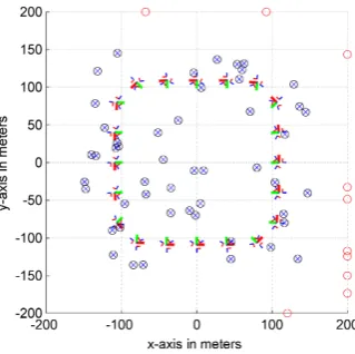
Parking lot simulation. We simulated a multi-camera system moving across a parking lot with loop closure, observing 50 scene points on the parking lot and 10 scene points far away at the hori-zon, i. e. at infinity (see Fig. 3). The multi-camera system con-tains three single-view cameras. Every scene point is observed by a camera ray on all 20 instances of time. The simulated set-up provides a high redundancy of observations. With a commonly

Figure 3: Simulation of a moving multi-camera system (poses shown as tripods) – e. g. on a parking lot – with loop closing. Scene points on the parking lot (crossed dots) and at the horizon (empty dots) being numerically at infinity are observed.

assumed standard deviation in the image plane of 0.3 pel and a camera constant with 500 pel, we add normally distributed noise withσl= 0.3/500radiant on the spherically normalized camera rays to simulate the observation process. As initial values for the bundle adjustment we randomly disturb both the generated spher-ical normalized homogeneous scene pointsXs

i by 10 % and the generated motion parametersR_{tandZtofMtby3}◦

and 2 meters respectively.

The iterative estimation procedure stops after six iterations, when the maximum normalized observation update is less than10−6

. The residuals of the observed image rays in the tangent space of the adjusted camera rays, which are approximately the radiant of small angles, do not show any deviation from the normal distribu-tion. The estimated a posteriori variance factor_bs0= 1.0021

ap-proves the a priori stochastic model with variance factorσ0 = 1.

Stereo camera data set. In order to test feasibility on real data we apply the bundle adjustment on 100 stereo images of a build-ing with a highly textured facade taken with the consumer stereo cameraFinePix Real 3D W3 from Fujifilm (see Fig. 4). We useAurelo without considering the known relative orientation between the stereo images to obtain an initial solution for the camera poses and the scene points. The dataset contains 284 813 image points and 12 439 observed scene points.

(a) left image (b) right image

Figure 4: Sample images of the stereo camera data set.

Starting from an a priori standard deviation for the image coordi-nates ofσl = 1pel, the a posteriori variance factor is estimated with _bs0 = 0.37indicating the automatically extracted Lowe

points to have an average precision of approximately 0.4 pel. The resulting scene points and the poses of the right stereo camera im-ages are shown in Fig. 5.

Figure 5: Illustration of the estimated scene points and poses of the right stereo camera images.

3.3 Decrease of rotational precision excluding far points

Bundle adjustment programs, such as Aurelo, cannot handle scene points with glancing intersections – e. g. with maximal in-tersection angles lower thanγ= 1gon – which therefore are ex-cluded in the estimation process to avoid numerical difficulties. Far scene points, however, can be observed over long periods of time and therefore should improve the quality of rotation estima-tion significantly. We investigate the decrease of precision of the estimated rotation parameters ofRb_twhen excluding scene points with glancing intersection angles. In detail, we will determine the average empirical standard deviationσαt =bs0

q

trΣRtcRtc/3for all estimated rotation parameters and report the average decrease of precision by excluding far points determined by the geomet-ric mean, namelyexphPT_t log(σαt/σ

′ αt)/T

i

, whereσ′ αt rep-resents the resulting average empirical standard deviation when scene points whose maximal intersection angle is lower than a thresholdγare excluded.

Parking lot simulation. We determine the decrease of preci-sion for the estimated rotation parameters by excluding a vary-ing number of scene points at infinity on the basis of the in Sec-tion 3.2 introduced simulaSec-tion of a moving multi-camera system on a parking lot. Again we generate 50 scene points close to the multi-camera positions and vary the number of scene points at in-finity to be 5, 10, 20, 50 and 100. The resulting average decrease in precision is 0.40 %, 2.31 %, 4.71 %, 7.03 % and 10.54 % re-spectively.

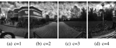
Multi-camera data set. We apply the bundle adjustment to an image sequence consisting of 360 images taken by four of the six cameras of the multi-camera systemLadybug 3(see Fig. 6). The Ladybug 3is mounted on a hand-guided platform and is triggered once per meter using an odometer. Approximate values are ob-tained with Aurelo by combining the individual cameras into a single virtual camera by adding distance dependent corrections on the camera rays, see Schmeing et al. (2011).

(a) c=1 (b) c=2 (c) c=3 (d) c=4

Figure 6: Sample images of the ladybug 3 data set.

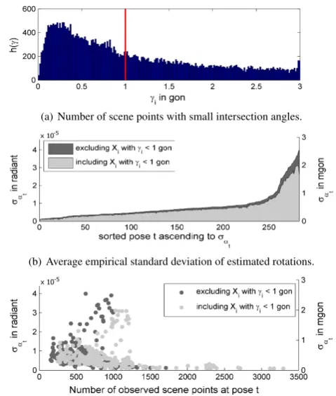
The data set contains 10 891 of 26 890 scene points observed with a maximal intersection angles per point significantly lower than

γ = 1gon, see the histogram in Fig. 7(a). The average stan-dard deviation of each estimated rotation parameter is shown in Fig. 7(b) showing the individual gain in precision that is mainly obtained due to a higher number of observed scene points at the individual poses, as can be seen in the scatter plot in Fig. 7(c). Some of the cameras show very large differences in the precision, demonstrating the relevance of the far scene points in the Lady-bug 3data set. Using far points results in an almost constant pre-cision of the rotation parameters over all camera stations, in con-trast to the results of the bundle adjustment excluding far points. The estimated a posteriori variance factor amountss_b0= 1.05

us-ing an a priori stochastic model withσl = 1pel for the image points, indicating a quite poor precision of the point detection which mainly results from the limited image quality.

Urban drive data set. We make the same investigation on an image sequence consisting of 283 images taken by a single-view camera mounted on a car. The data set contains 33 274 of 62 401 scene points observed with a maximal intersection angle per point smaller thanγ = 1gon, see Fig. 8(a). Excluding those scene points decreases the average precision of the estimated rotation parameters by about 17.41 %. The average standard deviation of each estimated rotation parameter is shown in Fig. 8(b) show-ing the individual gain in precision that again is mainly obtained due to a higher number of observed scene points at the individual poses, shown in scatter plot of Fig. 8(c). The estimated posteri-ori variance factor amountsbs0 = 0.54using a priori stochastic

model withσl= 1pel for the image points, indicating the preci-sion to be in a normal range.

4 CONCLUSIONS AND FUTURE WORK

We proposed a rigorous bundle adjustment for omnidirectional and multi-view cameras which enables an efficient maximum-likelihood estimation with image and scene points at infinity. Our experiments on simulated and real data sets show that scene points at the horizon stabilize the orientation of the camera rota-tions significantly. Future work will focus on solving the issue of estimating scene points like a church spire which is near to some cameras and for some others lying numerically at infinity. Furthermore we are developing a fast C-implementation and a concept for determining approximate values for the bundle ad-justment of multi-view cameras.

(a) Number of scene points with small intersection angles.

(b) Average empirical standard deviation of estimated rotations.

(c) Scatter plot ofσαtagainst the number of observed scene points att.

Figure 7: The histogram in (a) shows the number of scene points in the multi-camera dataset with small intersection angles. The average precision σαt determined by excluding and including scene points withγ < 1gon for all posest= 1, ..., T is com-pared to each other in (b) and against the number of observed scene points in (c).

Acknowledgements. This work was partially supported by the DFG-Project FOR 1505 ”Mapping on Demand”. The authors wish to thank the anonymous reviewers for their helpful com-ments.

References

Bartoli, A., 2002. On the Non-linear Optimization of Projective Motion Using Minimal Parameters. In: Proceedings of the 7th European Con-ference on Computer Vision-Part II, ECCV ’02, pp. 340–354.

F¨orstner, W., 2012. Minimal Representations for Uncertainty and Esti-mation in Projective Spaces. Zeitschrift f¨ur Photogrammetrie, Fern-erkundung und Geoinformation, Vol. 3, pp. 209–220.

Frahm, J.-M., K¨oser, K. and Koch, R., 2004. Pose estimation for Multi-Camera Systems. In: Mustererkennung ’04, Springer.

Hartley, R. I. and Zisserman, A., 2000. Multiple View Geometry in Com-puter Vision. Cambridge University Press.

Heuel, S., 2004. Uncertain Projective Geometry: Statistical Reasoning for Polyhedral Object Reconstruction. LNCS, Vol. 3008, Springer. PhD. Thesis.

Huber, P. J., 1981. Robust Statistics. John Wiley, New York.

Kanatani, K., 1996. Statistical Optimization for Geometric Computation: Theory and Practice. Elsevier Science.

Kim, J.-H., 2010. Camera Motion Estimation for Multi-Camera Systems. PhD thesis, School of Engineering, ANU College of Engineering and Computer Science, The Australian National University.

Kraus, K., 1997. Photogrammetry. D¨ummler Verlag Bonn. Vol.1: Fun-damentals and Standard Processes. Vol.2: Advanced Methods and Ap-plications.

(a) Number of scene points with small intersection angles.

(b) Average empirical standard deviation of estimated rotations.

(c) Scatter plot ofσαtagainst the number of observed scene points att.

Figure 8: The subplots (a), (b) and (c) show the results of the investigations explained in Fig. 7 on the urban drive dataset.

L¨abe, T. and F¨orstner, W., 2006. Automatic Relative Orientation of Im-ages. In: Proceedings of the 5th Turkish-German Joint Geodetic Days.

Lourakis, M. I. A. and Argyros, A. A., 2009. SBA: A Software Package for Generic Sparse Bundle Adjustment. ACM Transactions on Mathe-matical Software 36(1), pp. 1–30.

McGlone, C. J., Mikhail, E. M. and Bethel, J. S., 2004. Manual of Pho-togrammetry. American Society of Photogrammetry and Remote Sens-ing.

Meidow, J., Beder, C. and F¨orstner, W., 2009. Reasoning with Uncertain Points, Straight Lines, and Straight Line Segments in 2D. International Journal of Photogrammetry and Remote Sensing 64, pp. 125–139.

Mostafa, M. M. R. and Schwarz, K. P., 2001. Digital Image Georefer-encing from a Multiple Camera System by GPS/INS. PandRS 56(1), pp. 1–12.

Mouragnon, E., Lhuillier, M., Dhome, M. and Dekeyser, F., 2009. Generic and Real-time Structure from Motion Using Local Bundle Ad-justment. Image and Vision Computing 27(8), pp. 1178–1193.

Muhle, D., Abraham, S., Heipke, C. and Wiggenhagen, M., 2011. Esti-mating the Mutual Orientation in a Multi-Camera System with a Non Overlapping Field of View. In: Proceedings of the 2011 ISPRS Con-ference on Photogrammetric Image Analysis.

Nister, D., Naroditsky, O. and Bergen, J., 2004. Visual Odometry. In: IEEE Computer Society Conference on Computer Vision and Pattern Recognition, pp. 652–659.

Savopol, F., Chapman, M. and Boulianne, M., 2000. A Digital Multi CCD Camera System for Near Real-Time Mapping. In: Intl. Archives of Photogrammetry and Remote Sensing, Vol. XXXIII, Proc. ISPRS Congress, Amsterdam.

Schmeing, B., L¨abe, T. and F¨orstner, W., 2011. Trajectory Reconstruction Using Long Sequences of Digital Images From an Omnidirectional Camera. In: Proceedings of the 31th. DGPF Conference.