Manajemen | Fakultas Ekonomi Universitas Maritim Raja Ali Haji 073500103288619287

Full Terms & Conditions of access and use can be found at

http://www.tandfonline.com/action/journalInformation?journalCode=ubes20

Download by: [Universitas Maritim Raja Ali Haji] Date: 13 January 2016, At: 01:07

Journal of Business & Economic Statistics

ISSN: 0735-0015 (Print) 1537-2707 (Online) Journal homepage: http://www.tandfonline.com/loi/ubes20

Estimation of Dynamic Bivariate Mixture Models

Roman Liesenfeld & Jean-François Richard

To cite this article: Roman Liesenfeld & Jean-François Richard (2003) Estimation of Dynamic Bivariate Mixture Models, Journal of Business & Economic Statistics, 21:4, 570-576, DOI: 10.1198/073500103288619287

To link to this article: http://dx.doi.org/10.1198/073500103288619287

View supplementary material

Published online: 01 Jan 2012.

Submit your article to this journal

Article views: 45

Estimation of Dynamic Bivariate Mixture Models:

Comments on Watanabe (2000)

Roman L

IESENFELD

Department of Economics, Eberhard-Karls-Universität, Tübingen, Germany (roman.liesenfeld@uni-tuebingen.de)

Jean-François R

ICHARD

Department of Economics, University of Pittsburgh, Pittsburgh, PA (fantinC@pitt.edu)

This note compares a Bayesian Markov chain Monte Carlo approach implemented by Watanabe with a maximum likelihood ML approach based on an efŽcient importance sampling procedure to estimate dynamic bivariate mixture models. In these models, stock price volatility and trading volume are jointly directed by the unobservable number of price-relevant information arrivals, which is speciŽed as a serially correlated random variable. It is shown that the efŽcient importance sampling technique is extremely accurate and that it produces results that differ signiŽcantly from those reported by Watanabe.

KEY WORDS: Bayesian posterior means; EfŽcient importance sampling; Latent variable; Markov chain Monte Carlo; Maximum likelihood.

1. INTRODUCTION

Watanabe (2000) performed a Bayesian analysis of dynamic bivariate mixture models for the Nikkei 225 stock index fu-tures. Under these models, which were introduced by Tauchen and Pitts (1983) and modiŽed by Andersen (1996), stock price volatility and trading volume are jointly determined by the unobservable ow of price-relevant information arrivals. In particular, the high persistence in stock price volatility typ-ically found under autoregressive conditional heteroscedastic (ARCH) and stochastic volatility (SV) models is accounted for by serial correlation of the latent information arrival process. But because this process enters the models nonlinearly, the likelihood function and Bayesian posterior densities depend on high-dimensional interdependent integrals, whose evalua-tion requires the applicaevalua-tion of Monte Carlo (MC) integraevalua-tion techniques.

Watanabe (2000) used a Markov chain Monte Carlo (MCMC) integration technique, initially proposed by Jacquier, Polson, and Rossi (1994) in the context of univariate SV models. SpeciŽcally, he applied a variant of the Metropolis–Hasting acceptance-rejection algorithm proposed by Tierney (1994) (see also Chib and Greenberg 1995 for details) incorporating a multimove sampler proposed by Shephard and Pitt (1997). Details of this nontrivial algorithm were provided in appen-dix A of Watanabe’s article. Although Watanabe (2000) did not report computing times, the MCMC algorithm is computer-intensive (he used 18,000 draws for each integral evaluation), and assessing its convergence is delicate in the presence of highly correlated variables. Note, in particular, that his results pass a convergence diagnostics (CD) test proposed by Geweke (1992).

Watanabe’s Bayesian results for the bivariate mixture mod-els are distinctly at odds with results found in the literature for other datasets. SpeciŽcally, his estimates of volatility per-sistence are very close to those found for returns alone un-der univariate models. In contrast, the generalized method of moments (GMM) estimates obtained by Andersen (1996) for the U.S. stock market unequivocally indicate that persis-tence drops signiŽcantly under bivariate speciŽcations. This

Žnding is conŽrmed by the study of Liesenfeld (1998) for German stocks. Liesenfeld (1998) computed maximum like-lihood (ML) estimates using the accelerated Gaussian impor-tance sampling (AGIS) MC integration technique proposed by Danielsson and Richard (1993). This technique has since been generalized into an efŽcient importance sampling (EIS) procedure by Richard and Zhang (1996, 1997) and Richard (1998).

In this present article, we rely on the EIS procedure to rees-timate the Tauchen–Pitts model using Watanabe’s data. Our ML estimates and posterior means all differ signiŽcantly from Watanabe’s results and are fully consistent with the earlier Žnd-ings of Andersen (1996) and Liesenfeld (1998). We show that EIS likelihood estimates are numerically accurate even though they are based on as few as 50 MC draws. We also demon-strate that Watanabe’s results are the consequence of an appar-ent lack of convergence of the implemappar-ented MCMC algorithm in a single dimension of the parameter space. After discussions between the editors, Shephard, Watanabe, and ourselves, it now appears that the problem with Watanabe’s implementation of the multimove sampler originates from a typographical error in the work of Shephard and Pitt (1997). (A corrigendum to this ar-ticle is soon to appear inBiometrika.) In the meantime, Watan-abe has also corrected his own implementation and recently in-formed us that he now obtains results that are very similar to ours (see Watanabe and Omori 2002 for further details). Hence the focus of this article is to illustrate how EIS contributed to detecting a problem of an MCMC implementation that passed standard convergence tests. But EIS is more than just a proce-dure to check MCMC results—it is a powerful MC integration technique on its own that should be considered as a potential alternative to MCMC.

The remainder of the article is organized as follows. Sec-tion 2 briey reviews the bivariate mixture model of Tauchen

© 2003 American Statistical Association Journal of Business & Economic Statistics October 2003, Vol. 21, No. 4 DOI 10.1198/073500103288619287

570

Liesenfeld and Richard: Estimating Dynamic Bivariate Mixture Models 571

and Pitts (1983), and Section 3 outlines the EIS procedure. Sec-tion 4 compares the MCMC results of Watanabe (2000) for the Tauchen–Pitts model with those obtained by EIS. Tenta-tive explanations for the observed differences in these results are discussed. Section 5 summarizes our Žndings and con-cludes.

2. THE TAUCHEN–PITTS MODEL

Watanabe (2000) analyzed both the bivariate model of Tauchen and Pitts (1983) and a modiŽed version thereof, pro-posed by Andersen (1996). Because the salient features of both models are similar, here we discuss only the Tauchen and Pitts version, which is given by

RtjIt»N.0; ¾r2It/; (1) VtjIt»N.¹vIt; ¾v2It/; (2)

and

ln.It/DÁln.It¡1/C´t; ´t»N.0; ¾´2/; (3)

where Rt,Vt, andIt .t: 1!T/denote daily return, trading

volume, and unobservable number of information arrivals. The

´t’s are innovations, iid normally distributed. The model im-plies that,conditionallyon It,Rt andVt are normally

distrib-uted, independently from one another. Note that the conditional variance of returns as well as the conditional mean and vari-ance of volume are jointly driven by the common latent fac-torIt. Furthermore, the marginal distribution ofRtjItunder (1)

and (3) coincides with that implied by the standard univariate SV model. It is important to note that under the bivariate model (1)–(3), the volume series provides sample information on the latent processIt, and thus on the dynamics of the return process

itself.

Because the latent variableItis serially dependent, the

likeli-hood for the model (1)–(3) is given by aT-dimensional integral,

L.µIY/D

Z

f.Y;Xjµ /dX; (4)

where Y D fYtgT_tD1 and XD fXtgTtD1 denote the matrix of the observable variables Yt D.Rt;Vt/ and the vector of the

la-tent variable Xt Dln.It/. The integrand represents the joint

density ofY and X, indexed by the unknown parameter vec-tor µ D .¾r; Á; ¾´; ¹v; ¾v/0. No closed-form solutions exist

for the likelihood (4), nor can standard numerical integration procedures be applied. To estimate the dynamic Tauchen– Pitts model, Watanabe (2000) applied a MCMC technique that cycles between the distributions ofµjXt;Yt and Xtjµ ;Yt.

Under the noninformative prior density used by Watanabe (2000), the conditional distribution ofµjXt;Yt is obtained by

direct application of Bayes’s theorem, and sampling from it is straightforward. In contrast, sampling from the distribution of Xtjµ ;Yt requires a rather sophisticated application of the

acceptance-rejection technique, as described in Watanabe’s ap-pendix A.

3. EFFICIENT IMPORTANCE SAMPLING

The objective of this section is to provide a heuristic descrip-tion of EIS operadescrip-tion. Full technical and applicadescrip-tion details have been provided by Richard (1998) and Liesenfeld and Richard (2002). The integral in (4) can be written as

L.µIY/D whereg.¢/denotes the bivariate normal density associated with (1) and (2), andp.¢/denotes the density of the AR(1) process in (3). (For simulation purposes, one also must specify a dis-tribution for the initial conditionX0; this distinction is omitted here for ease of notation.) A simple MC estimate ofL.µIY/is

tD1 denotes a trajectory drawn from the se-quence ofp densities. SpeciŽcally,eX._ti/.µ / is drawn from the conditional densityp.XtjeX._t¡i/1.µ /; µ /. However, this simple pro-cedure completely ignores the fact that observation of theYt’s

conveys critical information on the underlying latent process. Therefore, the probability that a MC trajectory drawn from the

p process alone bears any resemblance to the actual (unob-served) sequence ofXt’s is 0 for all practical purposes. It

fol-lows that the MC estimator in (7) is hopelessly inefŽcient. [As documented by, e.g., Danielsson and Richard (1993), the range of values drawn for the term between brackets in Equation (7) often exceeds the computer oating point arithmetic capabili-ties.]

An EIS implementation starts with the selection of a se-quence of auxiliary samplersfm.XtjXt¡1;at/gT_tD1, typically de-Žned as a straightforward parametric extension of the initial samplersfp.XtjXt¡1; µ /gT_tD1 meant to capture sample informa-tion conveyed by theYt’s. For any choice of the auxiliary

para-metersat, the integral in (5) is rewritten as

L.µIY/

and the corresponding importance sampling (IS) MC likelihood estimate is given by quence of auxiliary (importance) samplersm.

EIS then aims to select values for theat’s that minimize the

MC sampling variance of the IS-MC likelihood estimate. This

requires achieving a good match between numerator and de-nominator in (9). Obviously, such a large-dimensional mini-mization problem must be broken down into manageable sub-problems. Note, however, that for any given value ofYt andµ,

the integral off.Yt;XtjXt¡1; µ /with respect toXt does depend

onXt¡1(which actually represents the density ofYtjXt¡1µ and is generally intractable), whereas that ofm.XtjXt¡1;at/equals 1

by deŽnition. Therefore, it is not possible to secure a good match between thef’s and them’s term by term.

Instead, EIS requires constructing a (positive) functional approximationk.Xt;Xt¡1Iat/ for the densityf.Yt;XtjXt¡1; µ / for any given .Yt; µ /, with the requirement that it be analyt-ically integrable with respect toXt. In Bayesian terminology, k.Xt;Xt¡1Iat/ serves as a density kernel for m.XtjXt¡1;at/,

which is then given by

m.XtjXt¡1;at/D

back into the periodt¡1 minimization subproblem. All in all, EIS requires solving a simple back-recursive sequence of low-dimensional least squares problems of the form

O version of (12) can be found in Richard 1998.] As in (7), feX._ti/.µ /gT

tD1denotes a trajectory drawn from the samplerp. (Al-thoughpis hopelessly inefŽcient for likelihood MC estimation, it generally sufŽces to produce a vastly improved IS sampler on a term by term least squares solution; a second and occasion-ally third iteration of the EIS algorithm, wherepis replaced by the previous stage IS sampler, sufŽces to produce a maximally efŽcient IS sampler.) The Žnal EIS estimate of the likelihood function is obtained by substitutingfOat.µ /gT_tD1forfatg

T

tD1in (9). [For implementation of the EIS procedure for the bivariate mix-ture model (1)–(3), see the Appendix.]

It turns out that EIS provides an exceptionally powerful tech-nique for the likelihood evaluation of (very) high-dimensional latent variables models. Our experience is that for such models, the integrand in (5) is a well-behaved function ofXgivenYand thus can be approximated with great accuracy by an importance sampler of the form given earlier, where the number of auxiliary parameters infatgT_tD1is proportional to the sample size. Likeli-hood functions for datasets consisting of several thousands ob-servations of daily Žnancial series have been accurately esti-mated with MC sample sizes no larger thanND50 (see, e.g., Liesenfeld and Jung 2000). In this article we useND50 MC

draws and 3 EIS iterations. Each EIS likelihood evaluation re-quires less than 1 second of computing time on a 733-MHz Pen-tium III PC for a code written in GAUSS; a full ML estimation, requiring approximately 25 BFGS iterations, takes of the order of 3 minutes.

In addition to its high accuracy, EIS offers a number of other key computational advantages:

1. Once the baseline algorithm in (12) has been programmed (which requires some attention in view of its recursive structure) changes in the model being analyzed require only minor modiŽcations of the code, generally only a few lines associated with the deŽnition of the functions enter-ing (12). For example, it took minimal adjustments in the program for the estimation of the univariate SV model (1) and (3) to obtain a corresponding code for the bivariate mixture model (1)–(3).

2. High accuracy in pointwise estimation of a likelihood function does not sufŽce to guarantee the convergence of a numerical optimizer, especially one using numerical gradients. Additional smoothing requires the application of the technique known as that of common random num-bers (CRNs), whereby allfeX._ti/.µ /gT_tD1draws for different values ofµ are obtained by transformation of a common set of canonical random numbersfeU._ti/gT

tD1, typically uni-forms or standardized normals. Note that such smoothing is also indispensable to secure the convergence of simu-lated MC estimates for a Žxed MC sample size (see, e.g., McFadden 1989; Pakes and Pollard 1989). This particu-lar issue is relevant when comparing EIS with MCMC. Whereas CRNs are trivially implementable in the context of EIS, in view of the typically simple form of the EIS samplers, it does not appear feasible to run MCMC under CRNs. Although this may not be critical for the compu-tation of Bayesian posterior moments, which requires in-tegration of the likelihood function rather than maximiza-tion, it does not appear feasible to numerically maximize a likelihood function estimated by MCMC at any level of generality.

3. Finally, because it takes only a few minutes to compute ML estimates, it is trivial to rerun the complete ML-EIS estimation under repeated draws ofYjX; µandXjY; µfor any value ofµ of interest (e.g., MC estimates or poste-rior means). Such reruns enable easy and cheap compu-tation of Žnite-sample estimates of the numerical (XjY), as well as statistical (YjX) accuracy of our parameter esti-mates (Bayesian or classical) (see Richard 1998 for addi-tional discussion and details). In the context of this article where, as discussed in Section 4, EIS produces results that are signiŽcantly different from those reported by Watan-abe (2000), these reruns are an essential component of our conclusion that there is a problem with Watanabe’s imple-mentation of the MCMC algorithm.

4. THE RESULTS

We estimated the SV model (1) and (3) as well as the dy-namic Tauchen–Pitts model (1)–(3) with the ML-EIS procedure for Watanabe’s data. The sample period starts on February 14,

Liesenfeld and Richard: Estimating Dynamic Bivariate Mixture Models 573

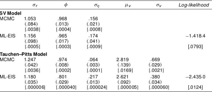
Table 1. MCMC and ML-EIS Estimation Results for the SV and Tauchen–Pitts Models

¾_r Á ¾´ ¹v ¾v Log-likelihood

SV Model

MCMC 1:053 :968 :156

.:084/ .:013/ .:021/

[:0038] [:0004] [:0008]

ML-EIS 1:156 :965 :174 ¡1;418:4

.:098/ .:017/ .:041/

[:0005] [:0003] [:0009] [.0793]

Tauchen–Pitts Model

MCMC 1:247 :974 :064 2:819 :669

.:042/ .:008/ .:003/ .:139/ .:029/

[:0036] [:0002] [:0001] [:0169] [:0021]

ML-EIS 1:180 :801 :217 2:621 :380 ¡2;435:0

.:035/ .:029/ .:013/ .:092/ .:034/

[:000006] [:000040] [:000024] [:000005] [:000060] [.0124]

NOTE: Asymptotic (statistical) standard errors are in parentheses, and MC (numerical) standard errors are in brackets. The MCMC posterior means and the MC standard errors of the posterior means are obtained from table 3 of Watanabe (2000). The MCMC posterior standard deviations are calculated from Watanbe’s draws from the posterior distribution. The ML-EIS estimates are based on a MC sample sizeND50 and three EIS iterations, and its asymptotic standard errors are obtained from a numerical approximation to the Hessian.

1994 and ends on October 1, 1997, giving a sample of 899 ob-servations. Whereas Watanabe (2000) computed Bayesian pos-terior means, we initially computed ML estimates. As we illus-trate, the actual differences between ML estimates and poste-rior means are very small, unsurprisingly in view of the facts that the likelihood functions of the models that we are consid-ering are very well-behaved, and that Watanabe (2000) used a noninformativeprior. His MCMC posterior means and standard deviations together with our ML-EIS estimates, are reported in Table 1.

For the SV model, the MCMC and ML-EIS results are very similar. In particular, the persistence parameterÁis estimated at .97 under both methods. Furthermore, both procedures exhibit similar degrees of numerical accuracy. This can be seen from a comparison of the MC (numerical) standard errors (for the ML-EIS estimates, they are obtained by Žtting the model 20 times under different sets of CRNs and computing the corresponding standard deviations).

In contrast, the divergence between the ML-EIS and Watan-abe results is striking for the Tauchen–Pitts model. In partic-ular, the ML-EIS method produces signiŽcantly smaller esti-mates of the persistence parameter,Á, and the variance para-meter for volume,¾v. In addition, the ML-EIS estimate for the variance parameter of the information arrival process,¾´, is

substantially larger than that reported by Watanabe (2000). It is important to note that the Žnding that the ML-EIS estimate of

Ádrops signiŽcantly (from .97 to .80) for the bivariate model is fully consistent with the GMM results of Andersen (1996) for a modiŽed version of the Tauchen–Pitts model estimated for U.S. stocks and with the ML-AGIS results of Liesenfeld (1998) for the Tauchen–Pitts speciŽcation for German stocks. In contrast, Watanabe’s MCMC posterior means ofÁ are nearly identical under both speciŽcations. Finally, it can be seen that the MC (numerical) standard errors for the ML-EIS estimates of the Tauchen–Pitts model are much smaller than those obtained for the univariate SV model. This makes perfect sense, because the EIS procedure applied to the bivariate model exploits the addi-tional information provided by the series of trading volumes on the behavior of the latent process.

Table 2 displays the estimated asymptotic correlation matrix for the ML-EIS estimates as obtained from a numerical approx-imation to the Hessian. Interestingly,the signs of the differences between the ML-EIS and Watanabe’s parameter estimates are the same as those of the corresponding correlations. For ex-ample, the ML-EIS estimator ofÁis positively correlated with that of¾vand negatively correlated with that of¾´. This is fully

consistent with the fact that a higher estimate ofÁby Watanabe coincides with a higher estimate of¾vand a lower estimate of ¾´relative to their corresponding ML-EIS counterparts.

First, we considered the possibility that be Žnite-sample bi-ases may be inherent in the ML-EIS estimation procedure. To address this concern, we conducted two simulation experiments in which we draw 100 Žctitious samples of size 899 from the Tauchen–Pitts model. In the Žrst experiment, the parameters were set equal to their ML-EIS estimates; in the second ex-periment, at their MCMC posterior means (as given in Table 1). ML-EIS estimates were then computed for each simulated sam-ple. MC means and standard deviations of the ML-EIS esti-mates under each set of parameter values are reported in Ta-ble 3. It is quite obvious that the ML-EIS estimation procedure performs very well under both sets of parameter values. Fur-thermore, it is worth noting that the Žnite-sample standard er-rors obtained under the ML-EIS parameter values are in very close agreement with the asymptotic standard errors of these estimates as given in Table 1.

We next considered the possibility that the log-likelihood function of the Tauchen–Pitts model might be at for this par-ticular dataset. Hence we Žrst computed the log-likelihood

Table 2. Estimated Correlation Matrix for the ML-EIS Estimates of the Tauchen–Pitts Model

¾r Á ¾´ ¹v ¾v

¾r 1:000 :076 ¡:094 :594 :197

Á 1:000 ¡:632 :074 :598

¾´ 1:000 ¡:114 ¡:776

¹v 1:000 :264

¾v 1:000

NOTE: The statistics are obtained from a numerical approximation to the Hessian.

Table 3. Mean and Standard Error of the ML-EIS Estimator for the Tauchen–Pitts Model

¾r Á ¾´ ¹v ¾v

True value 1:180 :801 :217 2:621 :380 Mean 1:183 :794 :217 2:622 :376 Standard error :030 :029 :014 :087 :035 True value 1:247 :974 :064 2:819 :669 Mean 1:249 :968 :065 2:811 :666 Standard error :048 :011 :007 :202 :030

NOTE: The statistics are based on 100 simulated samples, each consisting of a time series of length 899. The ML-EIS estimates are based on a MC sample sizeND50 and three EIS iterations.

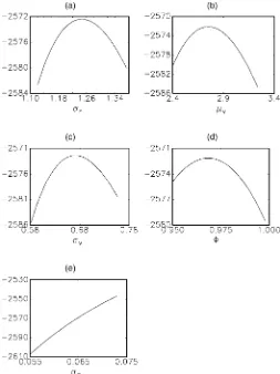
function at Watanabe’s posterior means and at our ML-EIS esti-mates. The correspondingvalues equal¡2;572:1 and¡2:435:0, implying a highly signiŽcant log-likelihooddifference of 137.1, immediately ruling out the possibility of a at log-likelihood function. This conclusion is supported by Figure 1, which shows sectional plots of the log-likelihood function at the ML-EIS parameter values. Obviously, the log-likelihoodis very well behaved around these estimates. Figure 2 displays similar plots at Watanabe’s posterior means. Note that whereas Watanabe’s posterior means are very far from our ML-EIS estimates, his posterior means of (¾r; Á; ¹v; ¾v) are close to maximizing a log-likelihood function in which¾´is set equal to its posterior

mean. In other words, Watanabe’s posterior means and the

ML-Figure 1. Sectional Log-Likelihood Functions for the Tauchen–Pitts Model at the ML-EIS Estimates of the Parameters: (a)¾r; (b)¹v; (c)¾v;

(d)Á; (e)¾´.

Figure 2. Sectional Log-Likelihood Functions for the Tauchen–Pitts Model at Watanabe’s MCMC Posterior Means of the Parameters: (a)¾_r; (b)¹_v; (c)¾_v; (d)Á; (e)¾´.

EIS estimates of these four parameters are fully consistent with one another,conditionallyon¾´. This does suggest that

Watan-abe’s initial algorithm might have got stuck in the¾´dimension

but converged in the four remaining dimensions.

Finally, to verify that ML estimates and posterior means are very close to one another for the well-behaved dataset, we calculated the posterior means based on the priors used by Watanabe using an IS technique. The posterior mean of the pa-rameter vectorµ D.¾r; Á; ¾´; ¹v; ¾v/0 is given by E.µjY/D

R

µL.µIY/p.µ /dµ =RL.µIY/p.µ /dµ. Hence, compared with the likelihood function, the integrals in the numerator and de-nominator ofE.µjY/exhibit Žve additional dimensions, one for each parameter. Watanabe adopted the following noninforma-tive priors for the elements ofµ:

p.¹v/DI[0;1]; p.Á/DI[¡1;1];

p.¾r//1=¾r; p.¾v//1=¾v; p.¾´//1=¾´;

whereI[a;b] is the indicator function of the interval [a;b]. If

m.µ /is an IS density forµ, then an importance MC estimate of

E.µjY/can be obtained as

bE.µjY/D 1

J

PJ jD1

£_Q

µ.j/eLN.µQ.j/IY/p.µQ.j//

¯

m.µQ.j//¤

1

J

PJ jD1

£

eLN.µQ.j/IY/p.µQ.j//

¯

m.µQ.j/_/¤ ;

Liesenfeld and Richard: Estimating Dynamic Bivariate Mixture Models 575

Table 4. Posterior Means Evaluated by Importance Sampling

¾_r Á ¾´ ¹v ¾v

Posterior mean 1:177 :816 :220 2:628 .354 MC standard error :034 :030 :018 :117 .032

NOTE: The posterior means are computed by using a MC sample size of 100, and the MC standard errors are obtained from 20 evaluations of the posterior means each based on a MC sample size of 100. The EIS evaluations of the likelihood are based on a MC sample sizeND50 and three EIS iterations.

wheref Qµ.j/gJ

jD1is a simulated sample ofJiid draws fromm.µ / andeLN.µQ.j/IY/is the value of the likelihood function at draw

Q

µ.j/obtained by the EIS procedure. An inspection of the sec-tional likelihood functions at the ML-EIS estimates ofµ (not presented here) revealed that they have shapes very similar to Gaussian densities. Hence we simply used a multivariate nor-mal distribution as importance samplerm.µ / with mean and variance given by the ML-EIS estimate ofµand the correspond-ing estimated asymptotic variance-covariance matrix. (Had we found that the posterior densities were less well behaved, we might have reprogrammed our EIS algorithm to include these Žve additional dimensions, but it was clearly not justiŽed here.) The IS MC estimates of the posterior means based on an MC sample size ofJD100, together with their MC standard er-rors, are reported in Table 4. Even though these estimates have relatively large MC standard errors (relative to the EIS stan-dards), they are sufŽciently accurate to conclude that all pos-terior means are very close to the ML-EIS estimates given in Table 1. All in all, we Žnd that the posterior densities of all Žve parameters are very well behaved for this dataset and cannot provide a rationale for the failure of Watanabe’s MCMC algo-rithm to converge in the¾´dimension.

5. CONCLUSIONS

We have estimated a dynamic bivariate mixture model with a ML procedure based on an EIS technique and obtained pa-rameter estimates that differ signiŽcantly from those reported by Watanabe (2000), who used a Bayesian MCMC multimove procedure for the same model and the same data set. Although our ML-EIS estimates are in accordance with the Žndings re-ported in the literature, Watanabe’s are at odds with those. In particular, his estimate of the persistence parameter of the latent information arrival process, which drives the joint dynamics of trading volume and return volatility, is signiŽcantly higher than the corresponding ML-EIS estimates, whereas his esti-mate of the variance parameter of the same process is much lower. Exploring possible explanations for these differences, we found that the ML estimates based on EIS are numeri-cally highly accurate. Moreover, it appears that although Watan-abe’s MCMC implementation fails to converge in the dimen-sion of the variance parameter of the latent information arrival process, his estimates of the four remaining parameters can be explained by the ML-EIS procedure. Because the observed dif-ferences in the estimates of the persistence and variance pa-rameter of the information arrival process are critical for an ex post analysis and forecasts of return volatility, we need to be particularly concerned about the possibility of implementa-tion errors. Whereas MCMC has repeatedly demonstrated its numerical capabilities across a wide range of applications, this

article ought to serve as a warning that MCMC implementa-tion problems might not be easily detectable. Note in particu-lar that Watanabe’s results did pass standard convergence tests. Obviously, the fact that we now have an alternative and pow-erful algorithm with EIS will help on this front. But EIS does more than just verify MCMC—it has repeatedly demonstrated high numerical accuracy, ease of implementation, and numer-ical stability. Also, its computational speed allows for running full simulation experiments to produce Žnite-sample measures of both numerical and statistical accuracy. Running such sim-ulation experiments with large sample sizes also provides an operational veriŽcation of the validity of any particular EIS implementation. In conclusion, EIS is deŽnitely an algorithm worthy of consideration on his exceptional numerical perfor-mance.

ACKNOWLEDGMENTS

The authors thank Toshiaki Watanabe for his very helpful and constructive cooperation, and former editor Jeffrey Wooldridge and an associate editor for their helpful comments.

APPENDIX: IMPLEMENTATION OF EFFICIENT IMPORTANCE SAMPLING FOR THE

TAUCHEN–PITTS MODEL

Computation of an EIS estimate of the likelihood function for the bivariate mixture model (1)–(3) for a given value of the parameter vectorµ requires the following steps:

Step (0). Draw a set ofN£Tindependent random numbers ffeU_t.i/gT

tD1g

N

iD1from a standardized normal distribution. These draws are used as CRNs during the complete EIS procedure to generate trajectories of the latent variable. Then use the ini-tial samplers p to draw N trajectories of the latent variable feX._ti/.µ /gT

tD1. According to (3) and (6), the initial samplers are characterized by the density of a Gaussian AR(1) process given by p.XtjXt¡1; µ //expf¡.Xt¡ÁXt¡1/2=2¾´2g, where

multi-plicative factors that do not depend onXtare omitted.

Step(t); (T:!1). Use the random draws from the initial samplers to solve the back-recursive sequence of the T least squares problems deŽned in (12). The relevant functional forms are obtained as follows. A natural choice for the auxiliary sam-plersmis to use parametric extensions of the initial samplers

p. This implies that the density kernel for the auxiliary sampler

m.XtjXt¡1;at/be a Gaussian density kernel forXt givenXt¡1,

which can be parameterized as

k.Xt;Xt¡1Iat/Dp.XtjXt¡1; µ /³ .Xt;at/; (A.1) where ³ is an auxiliary function given by ³ .Xt;at/ D

expfa1;tXtCa2;tXt2g, withatD.a1;t;a2;t/. Note that under this

parameterization, the initial samplerpcancels out in the least squares problem (12). Inserting the functional forms ofpand³

in (A.1) leads to the following form of the density kernels,

k.Xt;Xt¡1Iat//exp

where the conditional mean and variance of Xt on m are

given by

¹tD¾t2

Á

ÁXt¡1

¾2

´

Ca1;t

!

and ¾_t2D ¾

2

´

1¡2¾2

´a2;t

: (A.3)

Integratingk.Xt;Xt¡1Iat/with respect toXtleads to the

follow-ing form of the integratfollow-ing constant:

 .Xt¡1Iat//exp

»

¹2_t

2¾t2

¡.ÁXt¡1/ 2 2¾2

´

¼

; (A.4)

where irrelevant multiplicative factors are omitted.

Based on these functional forms, the steptleast squares prob-lem (12) is characterized by the linear auxiliary regression

lng¡YtjeXt.i/.µ /; µ

¢

Cln¡eXt.i/.µ /I OatC1.µ /

¢

DconstantCa1;teXt.i/.µ /Ca2;t

£_e

X_t.i/.µ /¤2

Cresidual; i: 1!N; (A.5)

whereg.¢/is the bivariate normal density forYt givenXt

asso-ciated with (1) and (2). The initial condition for the integrating constant is given by .XT;¢/´1.

Step (TC1). Use the Gaussian samplers fm.XtjXt¡1; O

at.µ //gT_tD1, which are characterized by the conditionalmean and variance given in (A.3), to drawNtrajectoriesfeX._ti/.aOt.µ //gT_tD1, from which the EIS estimate of the likelihood is calculated ac-cording to (9).

[Received August 2000. Revised November 2002.]

REFERENCES

Andersen, T. G. (1996), “Return Volatility and Trading Volume: An Informa-tion Flow InterpretaInforma-tion of Stochastic Volatility,”Journal of Finance, 51, 169–204.

Chib, S., and Greenberg, E. (1995), “Understanding the Metropolis–Hastings Algorithm,”The American Statistican, 49, 327–335.

Danielsson, J., and Richard, J. F. (1993), “Accelerated Gaussian Importance Sampler With Application to Dynamic Latent Variable Models,”Journal of Applied Econometrics, 8, S153–S173.

Geweke, J. (1992), “Evaluating the Accuracy of Sampling-Based Approaches to the Calculation of Posterior Moments,” inBayesian StatisticsVol. 4, eds. J. M. Bernardo, J. O. Berger, A. P. Dawid, and A. F. M. Smith, Oxford, U.K.: Oxford University Press, pp. 169–193.

Jacquier, E., Polson, N. G., and Rossi, P. E. (1994), “Bayesian Analysis of Sto-chastic Volatility Models,”Journal of Business & Economic Statistics, 12, 371–389.

Liesenfeld, R. (1998), “Dynamic Bivariate Mixture Models: Modeling the Be-havior of Prices and Trading Volume,”Journal of Business & Economic Sta-tistics, 16, 101–109.

Liesenfeld, R., and Jung, R. C. (2000), “Stochastic Volatility Models: Con-ditional Normality Versus Heavy-Tailed Distributions,”Journal of Applied Econometrics, 15, 137–160.

Liesenfeld, R., and Richard, J. F. (2002), “Univariate and Multivariate Stochas-tic Volatility Models: Estimation and DiagnosStochas-tics,”Journal of Empirical Fi-nance, forthcoming.

McFadden, D. (1989), “A Method of Simulated Moments for Estimation of Discrete Response Models Without Numerical Integration,”Econometrica, 57, 995–1026.

Pakes, A., and Pollard, D. (1989), “Simulation and the Asymptotics of Opti-mization Estimators,”Econometrica, 57, 1027–1058.

Richard, J. F. (1998), “EfŽcient High-Dimensional Monte Carlo Importance Sampling,” unpublished manuscript, University of Pittsburgh, Dept. of Eco-nomics.

Richard, J. F., and Zhang, W. (1996), “Econometric Modeling of UK House Prices Using Accelerated Importance Sampling,”The Oxford Bulletin of Eco-nomics and Statistics, 58, 601–613.

(1997), “Accelerated Monte Carlo Integration: An Application to Dy-namic Latent Variable Models,” inSimulation-Based Inference in Economet-rics: Methods and Application, eds. R. Mariano, M. Weeks, and T. Schuer-mann, Cambridge, U.K.: Cambridge University Press.

Shephard, N., and Pitt, M. (1997), “Likelihood Analysis of Non-Gaussian Measurement Time Series,” Biometrika, 84, 653–668; corr. forthcoming. (2003),x,xx.

Tauchen, G. E., and Pitts, M. (1983), “The Price Variability-Volume Relation-ship on Speculative Markets,”Econometrica, 51, 485–505.

Tierney, L. (1994), “Markov Chains for Exploring Posterior Distributions,”The Annals of Statistics, 21, 1701–1762.

Watanabe, T. (2000), “Bayesian Analysis of Dynamic Bivariate Mixture Mod-els: Can They Explain the Behavior of Returns and Trading Volume?,” Jour-nal of Business & Economic Statistics, 18, 199–210.

Watanabe, T., and Omori, Y. (2002), “Multi-Move Sampler for Estimating Non-Gaussian Time Series Models: Comments on Shephard and Pitt (1997),” unpublished manuscript, Tokyo Metropolitan University, Faculty of Eco-nomics.