ACCURACY COMPARISON OF DIGITAL SURFACE MODELS CREATED
BY UNMANNED AERIAL SYSTEMS IMAGERY AND TERRESTRIAL
LASER SCANNER
M. Naumann a *, M. Geist b, R. Bill a, F. Niemeyer a, G. Grenzdörffer a
a Rostock University, Professorship f. Geodesy & Geoinformatics, Germany - {matthias.naumann, ralf.bill,
frank.niemeyer, goerres.grenzdoerffer}@uni-rostock.de
b Large Structures in Production Engineering, Fraunhofer Application Center, 18059 Rostock, Germany -
KEY WORDS: DSM, 3D point cloud, UAS, TLS, Change Detection, Accuracy
ABSTRACT:
The main focus of the paper is a comparative study in which we have investigated, whether automatically generated digital surface models (DSM) obtained from unmanned aerial systems (UAS) imagery are comparable with DSM obtained from terrestrial laser scanning (TLS). The research is conducted at a pilot dike for coastal engineering. The effort and the achievable accuracy of both DSMs are compared. The error budgets of these two methods are investigated and the models obtained in each case compared against each other.
1. MOTIVATION
UAS do have the potential for rapid image acquisition of small areas from low altitudes and, in the sense of geometric point determination, from different viewing angles. Through waypoint navigation a full area coverage with large image overlap is possible. Sophisticated computation processes enable the automatic generation of 3D point clouds, DSM and ortho photos. Both the time and staff required for the entire processing chain, from image flight to DSM generation, is quite low.
The main focus of the paper is a comparative study in which we have investigated, whether automatically generated digital surface models (DSM) obtained from unmanned aerial systems (UAS) imagery are comparable with DSM obtained from terrestrial laser scanning (TLS). The research is conducted at a pilot dike for coastal engineering close to Rostock. The effort and the achievable accuracy of both DSM variants, derived from UAS based photogrammetry or obtained from terrestrial laser scanning (TLS), are compared and the differences are analysed in more detail.
For research topics, such as subsidence, consolidation and increased surface erosion, the comparison of high-resolution DSM from different times (change detection) is appropriate. Therefore, high-accurate and high-resolution DSMs are needed.
2. THE STUDY AREA
2.1 DredgDikes
The measurements took place at a test site – a dike, constructed in 2012 – located in Rostock Markgrafenheide. This dike is part of a research roject called DredgDikes. “The project DredgDikes was initiated by the University of Rostock (Prof. Fokke Saathoff) and Gdansk Technical University to investigate the application of dredged materials, geosynthetics and different
ashes in dike construction. The international cooperation is part-financed by the EU South Baltic Cross-border Cooperation Programme 2007-2013.
To investigate the different dredged materials and material combinations both in Rostock and Gdansk full scale test dikes have been built. A large number of measurements will be performed, including geotechnical field measurements, vegetation monitoring, measurements with respect to the release of contaminants (if needed), as well as seepage and overflowing tests.” (DredgDikes, 2013).
The dike (Figure 1) consists of four different material combinations with different dredged materials and geosynthetics. This pilot dike serves for multi-year large-scale field trials to test suitability of dewatered fine-grained, organic dredged material as a future cover layer for dike constructions.
The dike has a dimension of 40 x 140 m and connects 3 polders, which can be separately filled with water to simulate different hydraulic loads for over-flow and by-flow tests as well as water-logging measurements. To run a regular intensive monitoring program over the years and during the filling the test dike is equipped with a variety of geotechnical sensors (tensiometer, piezometer, Frequent Domain Reflectometry (FDR) sensors, meteorological station etc.). The geodetic measuring and monitoring program within the project consists of leveling and tacheometry for recurrent observation of selected points to detect deformations at these points.
Figure 1. Test dike in Rostock-Markgrafenheide (project DredgDikes, http://www.dredgdikes.eu/en/) International Archives of the Photogrammetry, Remote Sensing and Spatial Information Sciences, Volume XL-1/W2, 2013
2.2 Monitoring programme
The Chair of Geodesy and Geoinformatics (GG) at Rostock University decided to establish an additionally monitoring independent from the above mentioned geodetic and geotechnical monitoring program at the test dike, that could be used for investigations in two aspects:
1. Creation of a geodetic network with high precision from which periodic deformation measurements could be performed. This topic will not be treated in this paper.
2. Test new measurement methods such as terrestrial laser scanning (TLS) and image-based unmanned aerial system photogrammetry (UAS photogrammetry) to gauge their accuracy potential and to establish efficient workflows for measuring and evaluating.
2.2.1 Image based UAS: The size and extent of the test dike is well suited for the use of small UAS with little payload capacities (up to 1 kg) (Grenzdörffer et al., 2011, 2012). For data acquisition a MD4-1000 UAS from microdrones with a digital camera from Olympus (PEN e-P2) and a fixed focal length lens of 17 mm was used. In 2012 the area was surveyed four times: twice during the construction process of the dike and twice after finishing the construction. In 2013, two more UAS surveys were conducted. For the flight number 3, which is used for the comparison with the TLS, the flying height was around 85 to 90 m above ground. 3 flight strips are necessary to cover the test site, but we used 5 strips to capture the surrounding recorded. This results in a ground resolution of ca. 0.021 m per pixel. 11 ground control points (GCP) were arranged on and around the dike temporarily during the flight. They were used for geo-referencing the photogrammetric products. The 3D-positions of the GCPs have been determined by means of RTK-GPS with Leica GX1230 using the reference signals of SAPOS-HEPS (Satellite Positioning Service – High Precise Realtime Positioning Service). Their overall positioning mean error was determined by Leica GX1230 controller software (SmartWorx) and is about 0.013 m with a standard deviation of 0.004 m.
For geoprocessing of the imagery, state-of-the-art web processing service using Pix4UAV Cloud (Pix4UAV Cloud, 2013) and AgiSoft PhotoScan were used to compute the following photogrammetric products: 3D-point cloud, DSM and ortho photo mosaic. Pix4UAV Cloud computed the mean localisation error of the GCPs for flight with 0.008 m, 0.011 m and 0.013 m with a standard deviation of 0.006 m, 0.008 m and 0.005 m in their three coordinate directions East, North and Height in the new German coordinate reference system (ETRS89, UTM coordinates).
2.2.2 Terrestrial laser scanning: In addition terrestrial laser scanning was carried out together with the Fraunhofer AGP (Application Center for Large Structures in Production Engineering) with a delay of about three weeks to the corresponding UAS survey (Flight number 3). Scanning of the dike with its inner polders required 16 scanner locations. The IMAGER 5010i from Zoller + Fröhlich (Z+F) was used at a scan resolution of 3 mm per 10 meters.
The positions of the 13 temporarily targets, flat disks with a black & white marker laid out in the area of the test dike, were
determined with an average overall accuracy of about 1 cm with respect to a total station calibrated to the benchmark survey network. Additional 5 spherical targets were used for the scan to scan registration. All scans have been filtered by the preprocessing filters of the software LaserControl of Z+F. Only points with distance up to 30 m from the scanner position have been used for the DSM (reducing the influence of low angle of incidence). Furthermore, the pre-registration of the scans was calculated by the scanner software with a standard deviation of 0.003 m at the 13 target points (max. deviation 0.009 mm).
The co-registration of the partial scans was done by linking the individual measurement points to the reference coordinates and then computing a best-fit solution on identical areas in the scanning parts (minimizing the residuals). This was performed by using the software Polyworks of InnovMetric Software Inc. (InnovMetric, 2013) with a standard deviation of 2-3 mm.
3. RESULTS
3.1 Overall comparison
3.1.1 Preliminary remarks: After the completion of the dike construction, the UAS-DSM of the third period (flight number 3) was compared with the TLS-survey and the resulting DSM (TLS-DSM). For repeated measurements to be carried out in future, this is the reference epoch (epoch 0) for subsidence measurements. The measured surface areas were absolutely compared in the same coordinate reference system. Due to the latency of three weeks between UAS and TLS measurements some terrain changes in the adjacent area of the dike (mainly traffic movements, but also small construction activity) had taken place. Therefore, only the dike itself, and about 1 to 2 m from the adjacent area were included in our investigations.
In the comparisons each UAS surface element was assigned to the closest TLS surface element as a reference, since the TLS is regarded as a reference method based on the measurement arrangement. Instead differences along the Z-axis, the difference between next adjacent elements of the surfaces were compared. As a result, local height errors are not overstated, which result from measurement errors (e.g. on retaining walls), but there are the closest distances of the surfaces analyzed to each other.
First comparisons between the UAS- and TLS-DSMs showed good results with respect to the surface with a standard deviation of some cm (see 3.1.3). The biggest differences occured in places, where the dike was manually slightly reworked, e.g. installation of data cables, rakes the soil during the seeding (Figure 3). A more elaborate analysis (trimming of models) promises even better results, since parts of the DSMs (slope parts and cross sections) are used, which should be identical in reality. The error budgets of these two methods are investigated at a selection of planes and cross-sections over the dike. The models for these planes obtained in each case are compared against each other (see 3.2).
3.1.2 Time comparison for DSM capturing and modelling: The time required to capture such UAS DSM compared to conventional terrestrial surveying methods such as TLS DSM in our test area is about a factor 2 faster. For larger or more complex objects, the aforementioned factor may increase because more scanner locations were needed. Following is a listing of the required time expenses:
- UAS: Flight permit/flight planning and parameter settings 2 h, preparation of waypoint navigation 15 min, flight preparation at International Archives of the Photogrammetry, Remote Sensing and Spatial Information Sciences, Volume XL-1/W2, 2013
test site and RTK-GNSS surveying 30 min, flight accomplishment 15 min, pack up 15 min, data checking, measurement of GCP and DSM processing 2 h, in sum: 5,25 h. - TLS: Preparation and exploration of suitable scan stations 15 min, surveying of targets by tacheometry 45 min, data acquisition at least 15 min per station: 4 h, post processing divided into filtering: 1 h, feature-based and surface-based registration: 3 h (depends on software algorithm), creation and clean up of the polygon model: ≥ 1 h (depends on the number of iterations), in sum: 10,25 h.
3.1.3 Overall model: For the accuracy analysis in this paper we used the following colour codings (Figure 2).
Figure 2. Color schema legend for comparison of UAV-DSM minus TLS-DSM with a range of ±7.0 cm.
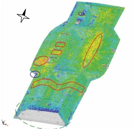
The magnitude of the surface deviations between the DSMs created by UAS and TLS are shown in Figure 3. Largely, they have a random character, in some areas smaller local systematic effects may be seen, which are caused by minor rework (ellipses: red=removal, blue=fill), greater reductions due to other surface structures (geo-textiles) or vegetation growth within the three weeks time offset.
Figure 3. Overall model with surface differences (view from south east). Areas with constructional reworks (ellipses),
areas with geo-textiles (polygones) and areas with greater vegetation growth (broken green line).
The empirical standard deviation of all the differences between the model surface is 0.040 m, leaving all outliers in the dataset (measure-ment errors, obstructions, etc.). If surface differences of greater than 10 cm are eliminated as erroneous measurements or outliers (0.67 %), the standard deviation can be reduced to 0.022 m (Table 1). Larger deviations were obtained with the UAS at objects of small area size or vertical surfaces, e.g. the construction walls at the overflow areas. This is caused by lower resolution and also due to errors in the detection of homologous points on the insufficiently textured construction walls. Compared to the TLS advantages in capturing areas on top of the dike and drainage ditches were detected. The TLS
showed slightly larger gaps here. This could be avoided by higher numbers of stations.
Without differences
exceeding 10 cm
All Differences
#Points 681338 685977
Mean [m] 0.000 0.000
StdDev [m] 0.022 0.040
Max dev. [m] 0.100 1.369
Min dev. [m] -0.100 -1.997
Table 1. Statistics of differences between UAS and TLS over the total extension (overall model)
3.2 Detailed accuracy analysis in parts of the models
The UAS and TLS models were selected and manually compared at 12 defined patches and 4 segments (Figure 4). The majority of the patches are limited by the walls of overflow areas of the western dike crowns. Further surfaces were evaluated on the levee crown, but also slope areas. Some of the results will be described here giving a representative view of the results.
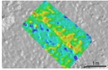
3.2.1 Segment analysis: In the three polders with their changing cross sections 4 segments, each one of 8 m width, were selected (Figure 4).
Figure 4. Selected patches and segments 1 to 4 (yellow band, numbered from south to north) used for accuracy comparisons
At these segments the deviations of UAS surface against the TLS surface were compared (Table 2) and visualized. In the compared segment 1 with 42543 points (Figure 5), the standard deviation of the surface differences is in the range of 0,022 m with an average error of 0,010 m (max. deviation: 0,274 m, min. deviation: -0,124 m).
Figure 5. Segment 1 (view from south) International Archives of the Photogrammetry, Remote Sensing and Spatial Information Sciences, Volume XL-1/W2, 2013
Seg. 1 Seg. 2 Seg. 3 Seg. 4
#Points 42543 45329 53128 37993
Mean [m] -0.010 -0.001 0.009 0.001 StdDev [m] 0.022 0.023 0.020 0.024 Max dev. [m] 0.274 0.212 0.271 0.234 Min dev. [m] -0.124 -0.239 -0.185 -0.321
Table 2. Statistics of differences between UAS and TLS for comparisons of the segments 1 to 4
Local rework on the dike surface can be easily recognized in this evaluation in segment 4, e.g. on top of the western dike side and in the bottom of the basin (Figure 6). Here we find the widest range of differences (max. minus min.) of the four segments. The differences in segment 4 were measured at 37993 points, this resulted in a standard deviation of 0.024 m with an average error of 0.001 m (max. deviation: 0.234 m, min. deviation: -0.321 m).
Figure 6. Segment 4 (view from south)
3.2.2 Plane analysis: At 12 plane surface elements, manually selected and delimited (embankment or dike), comparisons were carried out against best-fitting planes, which were calculated for these areas from the measured data. The criterion for the underlying regression analysis is to minimize the square error between the calculated and actual Z value (least squares method).
Figure 7. Deviations between UAS-DSM and the adjusted plane of the overflow surface 4 of the polder 2 (view from east)
Figure 8. Deviations between TLS-DSM and the adjusted plane of the overflow surface 4 of the polder 2 (view from east)
Measurements with residuals greater than 2 times the standard deviation were discarded to eliminate outliers (e.g. objects, people) in the scans. Figure 7 and 8 present a visual comparison of the surface analysis from both DSMs at the same overflow area. The deviations of both surfaces with respect to the adjusted planes are compared in table 3.
TLS UAS
#Points 9035 5795
Mean [m] 0.000 0.000
StdDev [m] 0.010 0.018
Max dev. [m] 0.038 0,130
Min dev. [m] -0.031 -0.078
#Points within +/-(1 * StdDev) 6664 (73.8%)
4612 (79.6%) #Points within +/-(2 * StdDev) 8464
(93.7%)
5596 (96.6%) #Points within +/-(3 * StdDev) 8981
(99.4%)
5703 (98.4%) #Points beyond +/-(3*StdDev) 54 92
Table 3. Deviations of both surfaces with respect to the adjusted planes of the overflow surface 4 of the polder 2
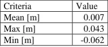
3.2.3 Assessment of the spatial position of the adjusted planes to each other: For each of the 12 planes differences between the two adjusted planes were calculated to assess the location and orientation in space to each other.
Figure 9. Differences between the adjusted planes (view from south-east)
For this purpose the adjusted planes were transformed from vector descriptions to a raster data set (equal grid size) and difference calculations between both grids of a test area were performed (Figure 9). They differ by an average of 0.007 cm (Table 4). The peak value is located in the reworked area of the polder 1.
Criteria Value
Mean [m] 0.007
Max [m] 0.043
Min [m] -0.062
Table 4. Results of the plane-to-plane-comparisons of 12 UAS-planes to TLS-UAS-planes
3.2.4 Small object analysis: In the areas around the retaining walls of the overflow areas relatively large errors in UAS-DSM were noticed. Average height errors in the order of several decimeters, in maximum even to the height of the wall (about 60 cm), occured in the area from 20 to 30 cm in front of the wall. Therefore, the surface tends to be too high, by approximately half the wall height. In contrast to the TLS-DSM, the differentiation of the wall as a sharply defined object is impossible in UAS-DSM (Figure 10).
Figure 10. Retaining wall of the overflow area 3 of polder 2, UAS-DSM in green and TLS-DSM in gray (perspective view
from the south)
On the west slope of polder 2 a change of curvature of the embankment surface could be detected in the UAS data as a terrain kink, resulting from a reduction of the width of the dike. Figure 11 shows the detected kink in both models. Figure 12 demonstrates the geometric principle.
Figure 11. Terrain kink in the transition area of polder 2 to polder 3 (planar view from east)
Figure 12. Principle sketches of the terrain kink and adjusted plane in planar view (left) and in cross section view (right)
The center buckling protrudes in both models in the range of about 3 cm with respect to the adjusted tangent planes in this investigation area. The differentiability is even better with the TLS measurements (Figure 13) due to their higher resolution, but the accuracy potential of the UAS model (Figure 14) could also be illustrated with this example (Table 5).
Figure 13. Detection of a terrain kink in the TLS model
Figure 14. Detection of a terrain kink in the UAS model
TLS UAS
#Points 20499 3118
Mean [m] 0.000 0.000
StdDev [m] 0.017 0.018
Max dev. [m] 0.101 0.068
Min dev. [m] -0.042 -0.090
#Points within +/-(1*StdDev) 13794 (67.3%)
2139 (68.6%) #Points within +/-(2*StdDev) 19808
(96.6%)
2994 (96.0%) #Points within +/-(3*StdDev) 20418
(99.6%)
3100 (99.4%) #Points beyond +-(3*StdDev) 81 18
Table 5. Deviations of both surfaces with respect to each adjusted plane at the investigation area „terrain kink“ at the
western embankment of polder 2
4. DISCUSSION
UAS photogrammetry and TLS scanning are different methods in geodesy for the generation of 3D models with high 3D accuracy. In our test object, which can be exemplary for other earthworks (coastal protection, road construction, landfill and open pits, mines), similar accuracies are achieved for both methods.
Under the assumption of similarity of objects in terms of comparable height extent, similar object complexity with less shading regions (more extended objects are conceivable) and similar vegetation conditions a similar accuracy potential for UAS-DSM as shown here can expected.
Our accuracy analysis showed that the UAS model is a little bit more inaccurate compared to the TLS model. There are two causes: on the one hand, the shape of the object with some technical installations (sharp edges, abrupt jumps in the height profile) and on the other hand, the lower resolution of the UAS-DSM. An accuracy improvement may be achieved with a lower flying height and by modification of the flight planning away from strips to more complex patterns. Redundancy in critical areas (shaded areas) could be increased hereby specifically. This is accompanied by the increase of flight time, using the example of the cross strips results in a doubling of the flight duration.
With TLS, the laser beam hits on a flat surface with increasing distance and more unfavorable to the object surface (abrasive cutting). TLS shows these problems in our implementation only on the dike lying areas. This effect can be partially mitigated but not resolved in principle, if the relative altitude of the scanner is increased with respect to this object, e.g. by higher settings of the scanner. This, however, also increases the technical effort as
1 m
1 m
stable constructions or equipments for the elevated viewpoints are necessary. In addition, for the analysis of TLS data different filters to reduce the influence of abrasive sections were developed, e.g. criteria for poor intersection angles or mixed-pixel filter. As a result of this filtering the need for further instrument points may occur and the effort increases. Despite these preventive measures due to the process of TLS derived DSMs the geometrical accuracy of different areas may vary (areas with inhomogeneous accuracy).
UAV shows in some places a lower resolution of the DSM and also inhomogeneous accuracy, for example vertical surfaces or steep embankments of trenches near the east side (not included in our investigation in this paper), which are poorly visible from above or can only be insufficiently linked. The already mentioned possibility to reduce the flying height provides a remedy here. Additionally the UAS could be flown directly along the trenches and in parallel with the walls.
In contrast to TLS, the measurements using UAS photogrammetry at adequate operational flight conditions ensures a stable and highly redundant geometric determination by favorable impact angles for most of the areas at the dike. The accuracy of the UAS DSM can therefore be more homogeneous than those of the TLS DSM, which is more dependent on individual scanner instrument points. Many parts of the dike were measured just once, only in the overlapping areas of multiple scans redundancies are present. Local factors such as abrasive cuts therefore act directly into the corresponding elevation data.
An essential prerequisite for UAS photogrammetry is the automated detection of tie points in the heterogeneous surface texture. Man-made surfaces with uniform color without distinctive texture cause misallocations in point link, so faulty positions and an incorrect model surface in these areas. The flying height and sufficiently bright but diffuse lighting conditions are also important. Shaded areas can present problems for point detection. The camera aperture is therefore set to a value that is a compromise with respect to the contrast of all image regions. Moreover, such exposure time should be chosen which prevents motion blur.
Depending on the dam height and the dam structure with larger height differences of course areas with different resolutions and attainable accuracies are achieved when flying at a constant altitude. This may result in problems at construction projects with greater height differences in the area of earthworks (e.g. landfill) or open pit. Varying the flying altitude may solve such problems. In the construction monitoring the flying route as well as the flying height may be adapted to the terrain conditions taking CAD plans into account.
With the use of web processing services for the UAS images, the user has no possibility of intervention on the calculation. So neither the process of filtering nor the meshing, can be controlled by parameters. Preference settings or interactions would be desirable in future releases.
5. REFERENCES
González-Aguilera, D., Fernández-Hernández, J., Mancera-Taboada, J., Rodríguez-Gonzálvez, P., Hernández-López, D., Felipe-García, B., Gozalo-Sanz, I., Arias-Perez, B., 2012. 3D Modelling and accuracy assessment of granite quarry using unmannend aerial vehicle. In: ISPRS (Int. Arch. Photogramm.
Remote Sens. Spatial Inf. Sci.), ISPRS Congress 2012, Melbourne, Australia, XXII ISPRS, 37-42.
Grenzdörffer, G., Niemeyer, F., 2011. UAV Based BRDF-Measurements of Agricultural Surfaces with PFIFFIKUS. In: Eisenbeiss, H. et al. [eds], Int. Arch. Photogramm. Remote Sens. Spatial Inf. Sci. Proceedings of the International Conference on Unmanned Aerial Vehicle in Geomatics (UAV-g), Zürich.
Grenzdörffer, G., Niemeyer, F., Schmidt, F., 2012. Development of Four Vision Camera System for a Micro UAV. ISPRS (Int. Arch. Photogramm. Remote Sens. Spatial Inf. Sci.), ISPRS Congress 2012, Melbourne, Australia, XXII ISPRS, S. 369–374.
DredgDikes:http://www.dredgdikes.eu/en/ (13.05.2013). Pix4UAV Cloud: http://pix4d.com/pix4uav_product.html (13.05.2013).
Agisoft: http://www.agisoft.ru (13.05.2013).
InnovMetric Software Inc.: http://www.innovmetric.com (13.05.2013)
ACKNOWLEDGEMENTS
The authors thank the Federal State of Mecklenburg-Western Pomerania for funding the project PFIFFikus (V220-630-08-TFMV-F-041).
The authors also thank the Fraunhofer Application Center for Large Structures in Production Engineering for their support during the TLS measurements and evaluations and the Chair of Environmental Geotechnics, Landscape Construction and Coastal Engineering at Rostock University for cooperation. International Archives of the Photogrammetry, Remote Sensing and Spatial Information Sciences, Volume XL-1/W2, 2013