• Tidak ada hasil yang ditemukan

PROBABILITY AND MATHEMATICAL STATISTICS (1)

N/A
N/A
Protected

Academic year: 2018

Membagikan "PROBABILITY AND MATHEMATICAL STATISTICS (1)"

Copied!
712
0
0

Teks penuh

(1)

PROBABILITY

AND

MATHEMATICAL STATISTICS

Prasanna Sahoo

(2)

THIS BOOK IS DEDICATED TO

AMIT

SADHNA

MY PARENTS, TEACHERS

AND

(3)
(4)
(5)
(6)

PREFACE

This book is both a tutorial and a textbook. This book presents an introduc-tion to probability and mathematical statistics and it is intended for students already having some elementary mathematical background. It is intended for a one-year junior or senior level undergraduate or beginning graduate level course in probability theory and mathematical statistics. The book contains more material than normally would be taught in a one-year course. This should give the teacher flexibility with respect to the selection of the content and level at which the book is to be used. This book is based on over 15 years of lectures in senior level calculus based courses in probability theory and mathematical statistics at the University of Louisville.

Probability theory and mathematical statistics are difficult subjects both for students to comprehend and teachers to explain. Despite the publication of a great many textbooks in this field, each one intended to provide an im-provement over the previous textbooks, this subject is still difficult to com-prehend. A good set of examples makes these subjects easy to understand. For this reason alone I have included more than 350 completely worked out examples and over 165 illustrations. I give a rigorous treatment of the fun-damentals of probability and statistics using mostly calculus. I have given great attention to the clarity of the presentation of the materials. In the text, theoretical results are presented as theorems, propositions or lemmas, of which as a rule rigorous proofs are given. For the few exceptions to this rule references are given to indicate where details can be found. This book contains over 450 problems of varying degrees of difficulty to help students master their problem solving skill.

(7)

are often worded in a confusing manner. They do not state the problem and then present the solution. Instead, they pass through a general discussion, never revealing what is to be solved for. In this book, I give many examples to illustrate each topic. Often we provide illustrations to promote a better understanding of the topic. All examples in this book are formulated as questions and clear and concise answers are provided in step-by-step detail.

There are several good books on these subjects and perhaps there is no need to bring a new one to the market. So for several years, this was circulated as a series of typeset lecture notes among my students who were preparing for the examination 110 of the Actuarial Society of America. Many of my students encouraged me to formally write it as a book. Actuarial students will benefit greatly from this book. The book is written in simple English; this might be an advantage to students whose native language is not English.

I cannot claim that all the materials I have written in this book are mine. I have learned the subject from many excellent books, such asIntroduction to Mathematical Statisticsby Hogg and Craig, andAn Introduction to Prob-ability Theory and Its Applicationsby Feller. In fact, these books have had a profound impact on me, and my explanations are influenced greatly by these textbooks. If there are some similarities, then it is due to the fact that I could not make improvements on the original explanations. I am very thankful to the authors of these great textbooks. I am also thankful to the Actuarial Society of America for letting me use their test problems. I thank all my students in my probability theory and mathematical statistics courses from 1988 to 2005 who helped me in many ways to make this book possible in the present form. Lastly, if it weren’t for the infinite patience of my wife, Sadhna, this book would never get out of the hard drive of my computer.

The author on a Macintosh computer using TEX, the typesetting system designed by Donald Knuth, typeset the entire book. The figures were gener-ated by the author using MATHEMATICA, a system for doing mathematics designed by Wolfram Research, and MAPLE, a system for doing mathemat-ics designed by Maplesoft. The author is very thankful to the University of Louisville for providing many internal financial grants while this book was under preparation.

(8)
(9)

TABLE OF CONTENTS

1. Probability of Events . . . 1 1.1. Introduction

1.2. Counting Techniques 1.3. Probability Measure

1.4. Some Properties of the Probability Measure 1.5. Review Exercises

2. Conditional Probability and Bayes’ Theorem . . . 27 2.1. Conditional Probability

2.2. Bayes’ Theorem 2.3. Review Exercises

3. Random Variables and Distribution Functions . . . 45 3.1. Introduction

3.2. Distribution Functions of Discrete Variables 3.3. Distribution Functions of Continuous Variables 3.4. Percentile for Continuous Random Variables 3.5. Review Exercises

4. Moments of Random Variables and Chebychev Inequality . 73 4.1. Moments of Random Variables

4.2. Expected Value of Random Variables 4.3. Variance of Random Variables 4.4. Chebychev Inequality

(10)

5. Some Special Discrete Distributions . . . 107 5.1. Bernoulli Distribution

5.2. Binomial Distribution 5.3. Geometric Distribution

5.4. Negative Binomial Distribution 5.5. Hypergeometric Distribution 5.6. Poisson Distribution

5.7. Riemann Zeta Distribution 5.8. Review Exercises

6. Some Special Continuous Distributions . . . 141 6.1. Uniform Distribution

6.2. Gamma Distribution 6.3. Beta Distribution 6.4. Normal Distribution 6.5. Lognormal Distribution 6.6. Inverse Gaussian Distribution 6.7. Logistic Distribution

6.8. Review Exercises

7. Two Random Variables . . . 185 7.1. Bivariate Discrete Random Variables

7.2. Bivariate Continuous Random Variables 7.3. Conditional Distributions

7.4. Independence of Random Variables 7.5. Review Exercises

8. Product Moments of Bivariate Random Variables . . . . 213 8.1. Covariance of Bivariate Random Variables

8.2. Independence of Random Variables

8.3. Variance of the Linear Combination of Random Variables 8.4. Correlation and Independence

(11)

9. Conditional Expectations of Bivariate Random Variables 237 9.1. Conditional Expected Values

9.2. Conditional Variance

9.3. Regression Curve and Scedastic Curves 9.4. Review Exercises

10. Functions of Random Variables and Their Distribution . 257 10.1. Distribution Function Method

10.2. Transformation Method for Univariate Case 10.3. Transformation Method for Bivariate Case

10.4. Convolution Method for Sums of Random Variables 10.5. Moment Method for Sums of Random Variables 10.6. Review Exercises

11. Some Special Discrete Bivariate Distributions . . . 289 11.1. Bivariate Bernoulli Distribution

11.2. Bivariate Binomial Distribution 11.3. Bivariate Geometric Distribution

11.4. Bivariate Negative Binomial Distribution 11.5. Bivariate Hypergeometric Distribution 11.6. Bivariate Poisson Distribution

11.7. Review Exercises

12. Some Special Continuous Bivariate Distributions . . . . 317 12.1. Bivariate Uniform Distribution

(12)

13. Sequences of Random Variables and Order Statistics . . 353 13.1. Distribution of Sample Mean and Variance

13.2. Laws of Large Numbers 13.3. The Central Limit Theorem 13.4. Order Statistics

13.5. Sample Percentiles 13.6. Review Exercises

14. Sampling Distributions Associated with

the Normal Population . . . 395 14.1. Chi-square distribution

14.2. Student’st-distribution 14.3. Snedecor’sF-distribution 14.4. Review Exercises

15. Some Techniques for Finding Point

Estimators of Parameters . . . 413 15.1. Moment Method

15.2. Maximum Likelihood Method 15.3. Bayesian Method

15.3. Review Exercises

16. Criteria for Evaluating the Goodness

of Estimators . . . 455 16.1. The Unbiased Estimator

16.2. The Relatively Efficient Estimator

16.3. The Minimum Variance Unbiased Estimator 16.4. Sufficient Estimator

(13)

17. Some Techniques for Finding Interval

Estimators of Parameters . . . 497 17.1. Interval Estimators and Confidence Intervals for Parameters 17.2. Pivotal Quantity Method

17.3. Confidence Interval for Population Mean 17.4. Confidence Interval for Population Variance

17.5. Confidence Interval for Parameter of some Distributions not belonging to the Location-Scale Family

17.6. Approximate Confidence Interval for Parameter with MLE 17.7. The Statistical or General Method

17.8. Criteria for Evaluating Confidence Intervals 17.9. Review Exercises

18. Test of Statistical Hypotheses . . . 541 18.1. Introduction

18.2. A Method of Finding Tests 18.3. Methods of Evaluating Tests

18.4. Some Examples of Likelihood Ratio Tests 18.5. Review Exercises

19. Simple Linear Regression and Correlation Analysis . . 585 19.1. Least Squared Method

19.2. Normal Regression Analysis 19.3. The Correlation Analysis 19.4. Review Exercises

20. Analysis of Variance . . . 621 20.1. One-way Analysis of Variance with Equal Sample Sizes

20.2. One-way Analysis of Variance with Unequal Sample Sizes 20.3. Pair wise Comparisons

(14)

21. Goodness of Fits Tests . . . 653 21.1. Chi-Squared test

21.2. Kolmogorov-Smirnov test 21.3. Review Exercises

(15)

Chapter 1

PROBABILITY OF EVENTS

1.1. Introduction

During his lecture in 1929, Bertrand Russel said, “Probability is the most important concept in modern science, especially as nobody has the slightest notion what it means.” Most people have some vague ideas about what prob-ability of an eventmeans. The interpretation of the wordprobabilityinvolves synonyms such as chance, odds, uncertainty, prevalence, risk, expectancy etc. “We use probability when we want to make an affirmation, but are not quite sure,” writes J.R. Lucas.

There are many distinct interpretations of the wordprobability. A com-plete discussion of these interpretations will take us to areas such as phi-losophy, theory of algorithm and randomness, religion, etc. Thus, we will only focus on two extreme interpretations. One interpretation is due to the so-called objective school and the other is due to the subjective school.

The subjective school defines probabilities as subjective assignments based on rational thought with available information. Some subjective prob-abilists interpret probabilities as the degree of belief. Thus, it is difficult to interpret the probability of an event.

(16)

Von Mises (1928) and Kolmogorov (1965). The Russian mathematician Kol-mogorov gave the solid foundation of probability theory using measure theory. The advantage of Kolmogorov’s theory is that one can construct probabilities according to the rules, compute other probabilities using axioms, and then interpret these probabilities.

In this book, we will study mathematically one interpretation of prob-ability out of many. In fact, we will study probprob-ability theory based on the theory developed by the late Kolmogorov. There are many applications of probability theory. We are studying probability theory because we would like to study mathematical statistics. Statistics is concerned with the de-velopment of methods and their applications for collecting, analyzing and interpreting quantitative data in such a way that the reliability of a con-clusion based on data may be evaluated objectively by means of probability statements. Probability theory is used to evaluate the reliability of conclu-sions and inferences based on data. Thus, probability theory is fundamental to mathematical statistics.

For an eventAof a discrete sample spaceS, the probability ofAcan be computed by using the formula

P(A) = N(A)

N(S)

where N(A) denotes the number of elements of A and N(S) denotes the number of elements in the sample spaceS. For a discrete case, the probability of an eventAcan be computed by counting the number of elements inAand dividing it by the number of elements in the sample spaceS.

In the next section, we develop various counting techniques. The branch of mathematics that deals with the various counting techniques is called combinatorics.

1.2. Counting Techniques

There are three basic counting techniques. They are multiplication rule, permutation and combination.

(17)

Example 1.1. Find the possible number of outcomes in a sequence of two tosses of a fair coin.

Answer: The number of possible outcomes is 2·2 = 4. This is evident from the following tree diagram.

H

T

H

T

H

T HH

HT

TH

TT

Tree diagram

Example 1.2. Find the number of possible outcomes of the rolling of a die and then tossing a coin.

Answer: Heren1= 6 andn2= 2. Thus by multiplication rule, the number of possible outcomes is 12.

Tree diagram 1 2 3 4 5 6

1H 1T 2H 2T 3H 3T 4H 4T 5H 5T 6H 6T H

T

Example 1.3. How many different license plates are possible if Kentucky uses three letters followed by three digits.

Answer:

(26)3(10)3

= (17576) (1000) = 17,576,000.

1.2.2. Permutation

(18)

a b c b a c c a b d a b a b d b a d c a d d a c a c b b c a c b a d b c a c d b c d c b d d b a a d c b d a c d b d c a a d b b d c c d a d c b

The number of possible ordered arrangements can be computed as follows: Since there are 3 positions and 4 objects, the first position can be filled in 4 different ways. Once the first position is filled the remaining 2 positions can be filled from the remaining 3 objects. Thus, the second position can be filled in 3 ways. The third position can be filled in 2 ways. Then the total number of ways 3 positions can be filled out of 4 objects is given by

(4) (3) (2) = 24.

In general, if r positions are to be filled from n objects, then the total number of possible ways they can be filled are given by

n(n1)(n2)· · ·(nr+ 1)

= n!

(nr)! =nPr.

Thus, nPr represents the number of ways r positions can be filled from n

objects.

Definition 1.1. Each of thenPr arrangements is called a permutation ofn

objects takenrat a time.

Example 1.4. How many permutations are there of all three of letters a, b, and c?

Answer:

3P3=

n! (n−r)! = 3!

(19)

Example 1.5. Find the number of permutations ofndistinct objects.

Answer:

nPn=

n! (nn)! =

n! 0! =n!.

Example 1.6. Four names are drawn from the 24 members of a club for the offices of President, Vice-President, Treasurer, and Secretary. In how many different ways can this be done?

Answer:

24P4=

(24)! (20)!

= (24) (23) (22) (21)

= 255,024.

1.2.3. Combination

In permutation, order is important. But in many problems the order of selection is not important and interest centers only on the set ofrobjects.

Let c denote the number of subsets of size r that can be selected from n different objects. The r objects in each set can be ordered in rPr ways.

Thus we have

nPr=c (rPr).

From this, we get

c= nPr

rPr

= n! (n−r)!r!

The numberc is denoted by!nr". Thus, the above can be written as

n

r ◆

= n! (n−r)!r!.

Definition 1.2. Each of the!nr"unordered subsets is called a combination ofnobjects takenrat a time.

(20)

Answer:

Thus 18 different committees can be formed.

1.2.4. Binomial Theorem

We know from lower level mathematics courses that

(x+y)2=x2+ 2xy+y2

In general, using induction arguments, we can show that

(x+y)n=

This result is called the Binomial Theorem. The coefficient!nk"is called the binomial coefficient. A combinatorial proof of the Binomial Theorem follows. If we write (x+y)n as thentimes the product of the factor (x+y), that is

(x+y)n = (x+y) (x+y) (x+y)· · ·(x+y), then the coefficient ofxn−kyk is!n

k

"

(21)

Remark 1.1. In 1665, Newton discovered the Binomial Series. The Binomial Series is given by

(1 +y)↵= 1 +

whereαis a real number and ✓α

k ◆

= α(α−1)(α−2)· · ·(α−k+ 1)

k! .

This!↵k"is called the generalized binomial coefficient.

Now, we investigate some properties of the binomial coefficients.

Theorem 1.1. Letn2N(the set of natural numbers) andr= 0,1,2, ..., n.

Proof: By direct verification, we get

n

This theorem says that the binomial coefficients are symmetrical.

Example 1.8. Evaluate!31"+!32"+!30".

(22)

Theorem 1.2. For any positive integernandr= 1,2,3, ..., n, we have

Equating the coefficients ofyr from both sides of the above expression, we

obtain

and the proof is now complete.

Example 1.9. Evaluate!2310"+!239"+!2411".

Example 1.10. Use the Binomial Theorem to show that

n

Answer: Using the Binomial Theorem, we get

(23)

for all real numbersx. Lettingx=−1 in the above, we get

Theorem 1.3. Letmandnbe positive integers. Then

k

Equating the coefficients of yk from the both sides of the above expression,

we obtain

and the conclusion of the theorem follows.

Example 1.11. Show that

(24)

Theorem 1.4. Letnbe a positive integer andk= 1,2,3, ..., n. Then

Proof: In order to establish the above identity, we use the Binomial Theorem together with the following result of the elementary algebra

xn−yn = (x−y)

Hence equating the coefficient ofxk, we obtain

n

This completes the proof of the theorem. The following result

(x1+x2+· · ·+xm)n=

(25)

This coefficient is known as the multinomial coefficient.

1.3. Probability Measure

A random experiment is an experiment whose outcomes cannot be pre-dicted with certainty. However, in most cases the collection of every possible outcome of a random experiment can be listed.

Definition 1.3. A sample space of a random experiment is the collection of all possible outcomes.

Example 1.12. What is the sample space for an experiment in which we select a rat at random from a cage and determine its sex?

Answer: The sample space of this experiment is

S={M, F}

whereM denotes the male rat andF denotes the female rat.

Example 1.13. What is the sample space for an experiment in which the state of Kentucky picks a three digit integer at random for its daily lottery?

Answer: The sample space of this experiment is

S={000,001,002,· · · ·,998,999}.

Example 1.14. What is the sample space for an experiment in which we roll a pair of dice, one red and one green?

Answer: The sample spaceS for this experiment is given by

S=

{(1,1) (1,2) (1,3) (1,4) (1,5) (1,6) (2,1) (2,2) (2,3) (2,4) (2,5) (2,6) (3,1) (3,2) (3,3) (3,4) (3,5) (3,6) (4,1) (4,2) (4,3) (4,4) (4,5) (4,6) (5,1) (5,2) (5,3) (5,4) (5,5) (5,6) (6,1) (6,2) (6,3) (6,4) (6,5) (6,6)} This setS can be written as

S ={(x, y)|1x6, 1y6}

(26)

Definition 1.4. Each element of the sample space is called a sample point.

Definition 1.5. If the sample space consists of a countable number of sample points, then the sample space is said to be a countable sample space.

Definition 1.6. If a sample space contains an uncountable number of sample points, then it is called a continuous sample space.

An eventAis a subset of the sample space S. It seems obvious that ifA andB are events in sample spaceS, thenA[B,Ac,A\B are also entitled

to be events. Thus precisely we define an event as follows:

Definition 1.7. A subsetAof the sample spaceSis said to be an event if it belongs to a collectionF of subsets ofS satisfying the following three rules: (a) S 2 F; (b) if A 2 F then Ac 2 F; and (c) if A

j 2 F for j ≥1, then

S1

j=12 F. The collectionF is called an event space or aσ-field. IfAis the

outcome of an experiment, then we say that the eventAhas occurred.

Example 1.15. Describe the sample space of rolling a die and interpret the event {1,2}.

Answer: The sample space of this experiment is

S={1,2,3,4,5,6}. The event{1,2}means getting either a 1 or a 2.

Example 1.16. First describe the sample space of rolling a pair of dice, then describe the eventAthat the sum of numbers rolled is 7.

Answer: The sample space of this experiment is

S={(x, y)|x, y= 1,2,3,4,5,6} and

A={(1,6),(6,1),(2,5),(5,2),(4,3),(3,4)}.

Definition 1.8. LetSbe the sample space of a random experiment. A prob-ability measureP : F ![0,1] is a set function which assigns real numbers to the various events ofS satisfying

(27)

(P3)P

1

[

k=1

Ak

! =

1

X

k=1

P(Ak)

ifA1, A2, A3, ..., Ak, ...are mutually disjoint events ofS.

Any set function with the above three properties is a probability measure forS. For a given sample spaceS, there may be more than one probability measure. The probability of an eventAis the value of the probability measure atA, that is

P rob(A) =P(A).

Theorem 1.5. If;is a empty set (that is an impossible event), then P(;) = 0.

Proof: LetA1=S andAi=;fori= 2,3, ...,1. Then

S=

1

[

i=1

Ai

whereAi\Aj =;fori6=j. By axiom 2 and axiom 3, we get

1 =P(S) (by axiom 2)

=P

1

[

i=1

Ai

!

=

1

X

i=1

P(Ai) (by axiom 3)

=P(A1) +

1

X

i=2

P(Ai)

=P(S) +

1

X

i=2

P(;)

= 1 +

1

X

i=2

P(;).

Therefore

1

X

i=2

P(;) = 0. SinceP(;)0 by axiom 1, we have

(28)

and the proof of the theorem is complete.

This theorem says that the probability of an impossible event is zero. Note that if the probability of an event is zero, that does not mean the event is empty (or impossible). There are random experiments in which there are infinitely many events each with probability 0. Similarly, if A is an event with probability 1, then it does not mean A is the sample space S. In fact there are random experiments in which one can find infinitely many events each with probability 1.

Theorem 1.6. Let {A1, A2, ..., An}be a finite collection of n events such

Proof: Consider the collection{A0

i}1i=1of the subsets of the sample spaceS

(29)

When n = 2, the above theorem yieldsP(A1[A2) = P(A1) +P(A2)

whereA1andA2are disjoint (or mutually exclusive) events.

In the following theorem, we give a method for computing probability of an event A by knowing the probabilities of the elementary events of the sample spaceS.

Theorem 1.7. If A is an event of a discrete sample space S, then the probability of A is equal to the sum of the probabilities of its elementary events.

Proof: Any setAinS can be written as the union of its singleton sets. Let

{Oi}1i=1 be the collection of all the singleton sets (or the elementary events)

ofA. Then

A=

1

[

i=1

Oi.

By axiom (P3), we get

P(A) =P

1

[

i=1

Oi

!

=

1

X

i=1

P(Oi).

Example 1.17. If a fair coin is tossed twice, what is the probability of getting at least one head?

Answer: The sample space of this experiment is

S={HH, HT, T H, T T}. The eventA is given by

A={at least one head} ={HH, HT, T H}.

By Theorem 1.7, the probability of A is the sum of the probabilities of its elementary events. Thus, we get

P(A) =P(HH) +P(HT) +P(T H)

=1 4+

1 4+

1 4

(30)

Remark 1.2. Notice that here we are not computing the probability of the elementary events by taking the number of points in the elementary event and dividing by the total number of points in the sample space. We are using the randomness to obtain the probability of the elementary events. That is, we are assuming that each outcome is equally likely. This is why the randomness is an integral part of probability theory.

Corollary 1.1. IfS is a finite sample space withnsample elements and A is an event inS withmelements, then the probability ofA is given by

P(A) =m n.

Proof: By the previous theorem, we get

P(A) =P

m

[

i=1

Oi

!

=

m

X

i=1

P(Oi)

=

m

X

i=1

1 n

= m n. The proof is now complete.

Example 1.18. A die is loaded in such a way that the probability of the face with j dots turning up is proportional toj for j = 1,2, ...,6. What is the probability, in one roll of the die, that an odd number of dots will turn up?

Answer:

P({j})/j =k j

wherekis a constant of proportionality. Next, we determine this constantk by using the axiom (P2). Using Theorem 1.5, we get

P(S) =P({1}) +P({2}) +P({3}) +P({4}) +P({5}) +P({6}) =k+ 2k+ 3k+ 4k+ 5k+ 6k

= (1 + 2 + 3 + 4 + 5 + 6)k

=(6)(6 + 1)

2 k

(31)

Using (P2), we get

21k= 1.

Thusk= 1

21. Hence, we have

P({j}) = j 21.

Now, we want to find the probability of the odd number of dots turning up.

P(odd numbered dot will turn up) =P({1}) +P({3}) +P({5}) = 1

21+ 3 21+

5 21

= 9 21.

Remark 1.3. Recall that the sum of the firstnintegers is equal to n

2(n+1).

That is,

1 + 2 + 3 +· · · ·+ (n2) + (n1) +n=n(n+ 1) 2 .

This formula was first proven by Gauss (1777-1855) when he was a young school boy.

Remark 1.4. Gauss proved that the sum of the first n positive integers is n(n+1)2 when he was a school boy. Kolmogorov, the father of modern probability theory, proved that the sum of the firstnodd positive integers is n2, when he was five years old.

1.4. Some Properties of the Probability Measure

Next, we present some theorems that will illustrate the various intuitive properties of a probability measure.

Theorem 1.8. IfA be any event of the sample spaceS, then

P(Ac) = 1P(A)

whereAc denotes the complement ofAwith respect toS.

Proof: LetA be any subset ofS. Then S=A[Ac. FurtherA andAc are

mutually disjoint. Thus, using (P3), we get

1 =P(S) =P(A[Ac)

(32)

A A c

Hence, we see that

P(Ac) = 1P(A). This completes the proof.

Theorem 1.9. IfA✓B✓S, then

P(A)P(B).

A

S

B

Proof: Note thatB =A[(B\A) where B\A denotes all the elementsx that are inB but not inA. Further,A\(B\A) =;. Hence by (P3), we get

P(B) =P(A[(B\A)) =P(A) +P(B\A).

By axiom (P1), we know thatP(B\A)0. Thus, from the above, we get P(B)P(A)

and the proof is complete.

Theorem 1.10. IfAis any event inS, then

(33)

Proof: Follows from axioms (P1) and (P2) and Theorem 1.8.

Theorem 1.10. IfAandB are any two events, then

P(A[B) =P(A) +P(B)−P(A\B).

Proof: It is easy to see that

A[B=A[(Ac\B)

and

A\(Ac\B) =;.

B A

S

Hence by (P3), we get

P(A[B) =P(A) +P(Ac\B) (1.1)

But the setB can also be written as

B= (A\B)[(Ac\B)

A

(34)

Therefore, by (P3), we get

P(B) =P(A\B) +P(Ac\B). (1.2)

EliminatingP(Ac\B) from (1.1) and (1.2), we get

P(A[B) =P(A) +P(B)P(A\B) and the proof of the theorem is now complete.

This above theorem tells us how to calculate the probability that at least one of AandB occurs.

Example 1.19. If P(A) = 0.25 and P(B) = 0.8, then show that 0.05 P(A\B)0.25.

Answer: SinceA\BAandA\BB, by Theorem 1.8, we get P(A\B)P(A) and also P(A\B)P(B). Hence

P(A\B)min{P(A), P(B)}. This shows that

P(A\B)0.25. (1.3) SinceA[B✓S, by Theorem 1.8, we get

P(A[B)P(S) That is, by Theorem 1.10

P(A) +P(B)P(A\B)P(S). Hence, we obtain

0.8 + 0.25P(A\B)1 and this yields

0.8 + 0.25−1P(A\B). From this, we get

(35)

From (1.3) and (1.4), we get

0.05P(A\B)0.25.

Example 1.20. Let A and B be events in a sample space S such that P(A) =1

2 =P(B) andP(Ac\Bc) = 1

3. Find P(A[Bc). Answer: Notice that

A[Bc=A[(Ac\Bc). Hence,

P(A[Bc) =P(A) +P(Ac\Bc) = 1

2+ 1 3

= 5 6.

Theorem 1.11. IfA1 andA2 are two events such thatA1✓A2, then

P(A2\A1) =P(A2)−P(A1).

Proof: The event A2can be written as

A2=A1

[

(A2\A1)

where the setsA1andA2\A1are disjoint. Hence

P(A2) =P(A1) +P(A2\A1)

which is

P(A2\A1) =P(A2)−P(A1)

and the proof of the theorem is now complete.

From calculus we know that a real function f : IR !IR (the set of real numbers) is continuous on IR if and only if, for every convergent sequence

{xn}1n=1 in IR,

lim

n!1f(xn) =f

⇣ lim

n!1xn

(36)

Theorem 1.12. IfA1, A2, ..., An, ...is a sequence of events in sample space

Proof: Given an increasing sequence of events

A1✓A2✓ · · · ✓An✓ · · ·

we define a disjoint collection of events as follows:

(37)

The second part of the theorem can be proved similarly.

Note that

lim

n!1An= 1

[

n=1

An

and

lim

n!1Bn= 1

\

n=1

Bn.

Hence the results above theorem can be written as

P⇣lim

n!1An

⌘ = lim

n!1P(An)

and

P⇣lim

n!1Bn

⌘ = lim

n!1P(Bn)

and the Theorem 1.12 is called the continuity theorem for the probability measure.

1.5. Review Exercises

1. If we randomly pick two television sets in succession from a shipment of 240 television sets of which 15 are defective, what is the probability that they will both be defective?

2. A poll of 500 people determines that 382 like ice cream and 362 like cake. How many people like both if each of them likes at least one of the two? (Hint: Use P(A[B) =P(A) +P(B)P(A\B) ).

3. The Mathematics Department of the University of Louisville consists of 8 professors, 6 associate professors, 13 assistant professors. In how many of all possible samples of size 4, chosen without replacement, will every type of professor be represented?

4. A pair of dice consisting of asix-sided die and a four-sided die is rolled and the sum is determined. Let A be the event that a sum of 5 is rolled and let B be the event that a sum of 5 or a sum of 9 is rolled. Find (a)P(A), (b) P(B), and (c)P(A\B).

(38)

6. Bill, George, and Ross, in order, roll a die. The first one to roll an even number wins and the game is ended. What is the probability that Bill will win the game?

7. LetAandBbe events such thatP(A) = 12=P(B) andP(Ac\Bc) =1 3.

Find the probability of the eventAc[Bc.

8. Suppose a box contains 4 blue, 5 white, 6 red and 7 green balls. In how many of all possible samples of size 5, chosen without replacement, will every color be represented?

9. Using the Binomial Theorem, show that

n

X

k=0

k ✓n

k ◆

=n2n−1.

10. A function consists of a domain A, a co-domain B and a rule f. The rulef assigns to each number in the domainAone and only one letter in the co-domainB. IfA={1,2,3}andB ={x, y, z, w}, then find all the distinct functions that can be formed from the setA into the setB.

11. LetS be a countable sample space. Let{Oi}1i=1 be the collection of all

the elementary events inS. What should be the value of the constantcsuch thatP(Oi) =c!13

"i

will be a probability measure inS?

12. A box contains five green balls, three black balls, and seven red balls. Two balls are selected at random without replacement from the box. What is the probability that both balls are the same color?

13. Find the sample space of the random experiment which consists of tossing a coin until the first head is obtained. Is this sample space discrete?

14. Find the sample space of the random experiment which consists of tossing a coin infinitely many times. Is this sample space discrete?

15. Five fair dice are thrown. What is the probability that a full house is thrown (that is, where two dice show one number and other three dice show a second number)?

16. If a fair coin is tossed repeatedly, what is the probability that the third head occurs on the nth toss?

(39)

18. An urn contains 3 red balls, 2 green balls and 1 yellow ball. Three balls are selected at random and without replacement from the urn. What is the probability that at least 1 color is not drawn?

19. A box contains four $10 bills, six $5 bills and two $1 bills. Two bills are taken at random from the box without replacement. What is the probability that both bills will be of the same denomination?

20. An urn containsnwhite counters numbered 1 throughn,nblack coun-ters numbered 1 through n, and n red counter numbered 1 through n. If two counters are to be drawn at random without replacement, what is the probability that both counters will be of the same color or bear the same number?

21. Two people take turns rolling a fair die. Person X rolls first, then personY, thenX, and so on. The winner is the first to roll a 6. What is the probability that personX wins?

22. Mr. Flowers plants 10 rose bushes in a row. Eight of the bushes are white and two are red, and he plants them in random order. What is the probability that he will consecutively plant seven or more white bushes?

23. Using mathematical induction, show that

dn

dxn[f(x)·g(x)] = n

X

k=0

n

k ◆ dk

dxk[f(x)]·

dn−k

(40)
(41)

Chapter 2

CONDITIONAL

PROBABILITIES

AND

BAYES’ THEOREM

2.1. Conditional Probabilities

First, we give a heuristic argument for the definition of conditional prob-ability, and then based on our heuristic argument, we define the conditional probability.

Consider a random experiment whose sample space is S. Let B ⇢ S. In many situations, we are only concerned with those outcomes that are elements ofB. This means that we considerB to be our new sample space.

B A

For the time being, suppose S is a nonempty finite sample space and B is a nonempty subset of S. Given this new discrete sample space B, how do we define the probability of an event A? Intuitively, one should define the probability of A with respect to the new sample space B as (see the figure above)

(42)

We denote the conditional probability ofAgiven the new sample spaceB as P(A/B). Hence with this notation, we say that

P(A/B) = N(A\B) N(B)

= P(A\B) P(B) ,

sinceN(S)6= 0. Here N(S) denotes the number of elements inS.

Thus, if the sample space is finite, then the above definition of the prob-ability of an event A given that the event B has occurred makes sense in-tuitively. Now we define the conditional probability for any sample space (discrete or continuous) as follows.

Definition 2.1. Let S be a sample space associated with a random exper-iment. The conditional probability of an event A, given that event B has occurred, is defined by

P(A/B) = P(A\B) P(B) providedP(B)>0.

This conditional probability measure P(A/B) satisfies all three axioms of a probability measure. That is,

(CP1)P(A/B)≥0 for all eventA (CP2)P(B/B) = 1

(CP3) IfA1, A2, ..., Ak, ...are mutually exclusive events, then

P(

1

[

k=1

Ak/B) = 1

X

k=1

P(Ak/B).

Thus, it is a probability measure with respect to the new sample spaceB.

Example 2.1. A drawer contains 4 black, 6 brown, and 8 olive socks. Two socks are selected at random from the drawer. (a) What is the probability that both socks are of the same color? (b) What is the probability that both socks are olive if it is known that they are of the same color?

Answer: The sample space of this experiment consists of

S={(x, y)|x, y2Bl, Ol, Br}. The cardinality ofS is

N(S) = ✓

18 2

(43)

LetAbe the event that two socks selected at random are of the same color. Then the cardinality ofAis given by

N(A) = ✓4

2 ◆

+ ✓6

2 ◆

+ ✓8

2 ◆

= 6 + 15 + 28

= 49.

Therefore, the probability ofAis given by

P(A) = !4918 2

" = 49 153.

Let B be the event that two socks selected at random are olive. Then the cardinality ofB is given by

N(B) = ✓8

2 ◆

and hence

P(B) = !8

2

" !18

2

" = 28 153.

Notice thatB A. Hence,

P(B/A) =P(A\B) P(A)

=P(B) P(A)

= ✓

28 153

◆ ✓ 153

49 ◆

=28 49 =

4 7.

LetA and B be two mutually disjoint events in a sample spaceS. We want to find a formula for computing the probability that the eventAoccurs before the eventBin a sequence trials. LetP(A) andP(B) be the probabil-ities that Aand B occur, respectively. Then the probability that neitherA norB occurs is 1−P(A)−P(B). Let us denote this probability byr, that isr= 1−P(A)−P(B).

(44)

IfB occurs in the first trial, then the probability ofAoccurs before B is 0. If neitherA nor B occurs in the first trial, we look at the outcomes of the second trial. In the second trial ifAoccurs, then the probability ofAoccurs beforeBis 1. IfBoccurs in the second trial, then the probability ofAoccurs before B is 0. If neither AnorB occurs in the second trial, we look at the outcomes of the third trial, and so on. This argument can be summarized in the following diagram.

P(A)

P(A)

P(A)

P(A)

A before B

A before B

A before B

A before B 1

1

1

1 0

0

0

0

P(B)

P(B)

P(B)

P(B) r = 1-P(A)-P(B)

r r

r r

Hence the probability that the eventAcomes before the eventB is given by

P(A before B) =P(A) +r P(A) +r2P(A) +r3P(A) +· · ·+rnP(A) +· · ·

=P(A) [1 +r+r2+· · ·+rn+· · ·] =P(A) 1

1r

=P(A) 1

1−[1−P(A)−P(B)] = P(A)

P(A) +P(B).

The eventAbeforeB can also be interpreted as a conditional event. In this interpretation the event Abefore B means the occurrence of the event Agiven thatA[B has already occurred. Thus we again have

P(A/A[B) = P(A\(A[B)) P(A[B) = P(A)

P(A) +P(B).

(45)

Answer: The sample space of this random experiment is

S=

{(1,1) (1,2) (1,3) (1,4) (2,1) (2,2) (2,3) (2,4) (3,1) (3,2) (3,3) (3,4) (4,1) (4,2) (4,3) (4,4)}.

Let A denote the event of getting a sum of 3 and B denote the event of getting a sum of 5. The probability that a sum of 3 is rolled before a sum of 5 is rolled can be thought of as the conditional probability of a sum of 3, given that a sum of 3 or 5 has occurred. That is,P(A/A[B). Hence

P(A/A[B) = P(A\(A[B)) P(A[B) = P(A)

P(A) +P(B)

= N(A) N(A) +N(B)

= 2 2 + 4

= 1 3.

Example 2.3. If we randomly pick two television sets in succession from a shipment of 240 television sets of which 15 are defective, what is the proba-bility that they will be both defective?

Answer: LetAdenote the event that the first television picked was defective. LetBdenote the event that the second television picked was defective. Then A\Bwill denote the event that both televisions picked were defective. Using the conditional probability, we can calculate

P(A\B) =P(A)P(B/A) =

✓ 15 240

◆ ✓ 14 239

= 7 1912.

In Example 2.3, we assume that we are sampling without replacement.

(46)

Rolling a die is equivalent to sampling with replacement, whereas dealing a deck of cards to players is sampling without replacement.

Example 2.4. A box of fuses contains 20 fuses, of which 5 are defective. If 3 of the fuses are selected at random and removed from the box in succession without replacement, what is the probability that all three fuses are defective?

Answer: LetA be the event that the first fuse selected is defective. LetB be the event that the second fuse selected is defective. LetC be the event that the third fuse selected is defective. The probability that all three fuses selected are defective isP(A\B\C). Hence

P(A\B\C) =P(A)P(B/A)P(C/A\B) =

5

20 ◆ ✓4

19 ◆ ✓ 3

18 ◆

= 1 114.

Definition 2.3. Two eventsAand B of a sample spaceS are called inde-pendent if and only if

P(A\B) =P(A)P(B).

Example 2.5. The following diagram shows two events A and B in the sample spaceS. Are the eventsAandB independent?

A

B

S

Answer: There are 10 black dots inS and eventAcontains 4 of these dots. So the probability of A, is P(A) = 104. Similarly, event B contains 5 black dots. HenceP(B) = 105. The conditional probability ofAgivenB is

P(A/B) =P(A\B) P(B) =

(47)

This shows thatP(A/B) =P(A). HenceA andB are independent.

Theorem 2.1. Let A, B S. If Aand B are independent and P(B)>0, then

P(A/B) =P(A).

Proof:

P(A/B) =P(A\B) P(B)

=P(A)P(B) P(B) =P(A).

Theorem 2.2. If A and B are independent events. Then Ac and B are

independent. SimilarlyAandBc are independent.

Proof: We know thatA andB are independent, that is

P(A\B) =P(A)P(B)

and we want to show thatAc andB are independent, that is

P(Ac\B) =P(Ac)P(B). Since

P(Ac\B) =P(Ac/B)P(B) = [1P(A/B)]P(B) =P(B)P(A/B)P(B) =P(B)−P(A\B) =P(B)P(A)P(B) =P(B) [1−P(A)] =P(B)P(Ac),

the eventsAcandB are independent. Similarly, it can be shown thatAand

Bc are independent and the proof is now complete.

(48)

that it should be interpreted by the rule of multiplication of probabilities and this leads to the mathematical definition of independence.

Example 2.6. Flip a coin and then independently cast a die. What is the probability of observing heads on the coin and a 2 or 3 on the die?

Answer: LetAdenote the event of observing a head on the coin and letB be the event of observing a 2 or 3 on the die. Then

Example 2.7. An urn contains 3 red, 2 white and 4 yellow balls. An ordered sample of size 3 is drawn from the urn. If the balls are drawn with replacement so that one outcome does not change the probabilities of others, then what is the probability of drawing a sample that has balls of each color? Also, find the probability of drawing a sample that has two yellow balls and a red ball or a red ball and two white balls?

Answer:

If the balls are drawn without replacement, then

P(RW Y) =

There is a tendency to equate the concepts “mutually exclusive” and “inde-pendence”. This is a fallacy. Two eventsA andB are mutually exclusiveif A\B=;and they are calledpossibleifP(A)6= 06=P(B).

(49)

Proof: Suppose not. Then

P(A\B) =P(A)P(B) P(;) =P(A)P(B) 0 =P(A)P(B).

Hence, we get either P(A) = 0 or P(B) = 0. This is a contradiction to the fact thatAandB are possible events. This completes the proof.

Theorem 2.3. Two possible independent events are not mutually exclusive.

Proof: Let A andB be two independent events and supposeA andB are mutually exclusive. Then

P(A)P(B) =P(A\B) =P(;) = 0.

Therefore, we get either P(A) = 0 or P(B) = 0. This is a contradiction to the fact thatAandB are possible events.

The possible eventsAandBexclusive impliesAandB are not indepen-dent; andAandB independent impliesAandB are not exclusive.

2.2. Bayes’ Theorem

There are many situations where the ultimate outcome of an experiment depends on what happens in various intermediate stages. This issue is re-solved by the Bayes’ Theorem.

Definition 2.4. LetSbe a set and letP ={Ai}mi=1be a collection of subsets

ofS. The collectionP is called a partition ofS if (a) S=

m

[

i=1

Ai

(b) Ai\Aj=; fori6=j.

Sample A1

A2

A3 A4

A5

(50)

Theorem 2.4. If the events {Bi}mi=1 constitute a partition of the sample

spaceS andP(Bi)6= 0 fori= 1,2, ..., m, then for any eventAinS

P(A) =

m

X

i=1

P(Bi)P(A/Bi).

Proof: Let S be a sample space and A be an event inS. Let {Bi}mi=1 be

any partition ofS. Then

A=

m

[

i=1

(A\Bi).

Thus

P(A) =

m

X

i=1

P(A\Bi)

=

m

X

i=1

P(Bi)P(A/Bi).

Theorem 2.5. If the events {Bi}mi=1 constitute a partition of the sample

space S and P(Bi) 6= 0 for i = 1,2, ..., m, then for any event A inS such

thatP(A)6= 0

P(Bk/A) =

P(Bk)P(A/Bk)

Pm

i=1P(Bi)P(A/Bi)

k= 1,2, ..., m.

Proof: Using the definition of conditional probability, we get

P(Bk/A) =

P(A\Bk)

P(A) .

Using Theorem 1, we get

P(Bk/A) =

P(A\Bk)

Pm

i=1P(Bi)P(A/Bi)

.

This completes the proof.

This Theorem is called Bayes Theorem. The probabilityP(Bk) is called

prior probability. The probabilityP(Bk/A) is called posterior probability.

(51)

marbles. Box B2 contains 3 green marbles and 10 yellow marbles. The

boxes are arranged so that the probability of selecting box B1 is 13 and the

probability of selecting boxB2is 23. Kathy is blindfolded and asked to select

a marble. She will win a color TV if she selects a green marble. (a) What is the probability that Kathy will win the TV (that is, she will select a green marble)? (b) If Kathy wins the color TV, what is the probability that the green marble was selected from the first box?

Answer: LetA be the event of drawing a green marble. The prior proba-bilities areP(B1) =13 andP(B2) =23.

(a) The probability that Kathy will win the TV is

P(A) =P(A\B1) +P(A\B2)

=P(A/B1)P(B1) +P(A/B2)P(B2)

= ✓7

11 ◆ ✓1

3 ◆

+ ✓3

13 ◆ ✓2

3 ◆

= 7 33+

2 13

= 91 429+

66 429

= 157 429.

(b) Given that Kathy won the TV, the probability that the green marble was selected fromB1is

1/3

2/3

Selecting box B1

Selecting box B2

Green marble

Not a green marble Green marble

Not a green marble 7/11

(52)

P(B1/A) =

P(A/B1)P(B1)

P(A/B1)P(B1) +P(A/B2)P(B2)

=

!7 11

" !1 3

" !7

11

" !1 3

"

+!133" !23"

= 91 157.

Note that P(A/B1) is the probability of selecting a green marble from

B1 whereasP(B1/A) is the probability that the green marble was selected

from boxB1.

Example 2.9. Suppose box A contains 4 red and 5 blue chips and boxB contains 6 red and 3 blue chips. A chip is chosen at random from the boxA and placed in boxB. Finally, a chip is chosen at random from among those now in boxB. What is the probability a blue chip was transferred from box Ato boxB given that the chip chosen from boxB is red?

Answer: LetErepresent the event of moving a blue chip from boxAto box B. We want to find the probability of a blue chip which was moved from box A to box B given that the chip chosen fromB was red. The probability of choosing a red chip from boxAisP(R) =49 and the probability of choosing a blue chip from boxAisP(B) =5

9. If a red chip was moved from boxAto

box B, then box B has 7 red chips and 3 blue chips. Thus the probability of choosing a red chip from boxB is 7

10. Similarly, if a blue chip was moved

from box Ato box B, then the probability of choosing a red chip from box B is 6

10.

blue 5/9

Red chip

Not a red chip

Red chip

Not a red chip red 4/9

Box A

Box B 7 red 3 blue

Box B 6 red 4 blue

3/10 7/10

6/10

(53)

Hence, the probability that a blue chip was transferred from boxAto boxB given that the chip chosen from boxB is red is given by

P(E/R) =P(R/E)P(E) P(R)

=

!6 10

" !5 9

" !7

10

" !4 9

"

+!106" !59"

=15 29.

Example 2.10. Sixty percent of new drivers have had driver education. During their first year, new drivers without driver education have probability 0.08 of having an accident, but new drivers with driver education have only a 0.05 probability of an accident. What is the probability a new driver has had driver education, given that the driver has had no accident the first year?

Answer: LetArepresent the new driver who has had driver education and B represent the new driver who has had an accident in his first year. LetAc

and Bc be the complement of A and B, respectively. We want to find the

probability that a new driver has had driver education, given that the driver has had no accidents in the first year, that isP(A/Bc).

P(A/Bc) =P(A\Bc)

P(Bc)

= P(B

c/A)P(A)

P(Bc/A)P(A) +P(Bc/Ac)P(Ac)

= [1−P(B/A)]P(A)

[1P(B/A)]P(A) + [1P(B/Ac)] [1P(A)]

=

!60 100

" !95 100

" !40

100

" !92 100

"

+!10060" !10095"

= 0.6077.

(54)

have AIDS but the test is not perfect. For people with AIDS, the test misses the diagnosis 2% of the times. And for the people without AIDS, the test incorrectly tells 3% of them that they have AIDS. (a) What is the probability that a person picked at random will test positive? (b) What is the probability that you have AIDS given that your test comes back positive?

Answer: LetAdenote the event of one who has AIDS and letB denote the event that the test comes out positive.

(a) The probability that a person picked at random will test positive is given by

P(test positive) = (0.005) (0.98) + (0.995) (0.03)

= 0.0049 + 0.0298 = 0.035.

(b) The probability that you have AIDS given that your test comes back positive is given by

P(A/B) =favorable positive branches total positive branches

= (0.005) (0.98)

(0.005) (0.98) + (0.995) (0.03)

=0.0049

0.035 = 0.14.

0.995 AIDS

Test positive

Test negative

Test positive

Test negative 0.98

0.02

0.03 0.005

0.97 No AIDS

(55)

2.3. Review Exercises

1. LetP(A) = 0.4 andP(A[B) = 0.6. For what value ofP(B) are Aand B independent?

2. A die is loaded in such a way that the probability of the face withj dots turning up is proportional tojforj= 1,2,3,4,5,6. In 6 independent throws of this die, what is the probability that each face turns up exactly once?

3. A system engineer is interested in assessing the reliability of a rocket composed of three stages. At take off, the engine of the first stage of the rocket must lift the rocket off the ground. If that engine accomplishes its task, the engine of the second stage must now lift the rocket into orbit. Once the engines in both stages 1 and 2 have performed successfully, the engine of the third stage is used to complete the rocket’s mission. The reliability of the rocket is measured by the probability of the completion of the mission. If the probabilities of successful performance of the engines of stages 1, 2 and 3 are 0.99, 0.97 and 0.98, respectively, find the reliability of the rocket.

4. Identical twins come from the same egg and hence are of the same sex. Fraternal twins have a 50-50 chance of being the same sex. Among twins the probability of a fraternal set is 1

3 and an identical set is 2

3. If the next set of

twins are of the same sex, what is the probability they are identical?

5. In rolling a pair of fair dice, what is the probability that a sum of 7 is rolled before a sum of 8 is rolled ?

6. A card is drawn at random from an ordinary deck of 52 cards and re-placed. This is done a total of 5 independent times. What is the conditional probability of drawing the ace of spades exactly 4 times, given that this ace is drawn at least 4 times?

7. LetAandB be independent events withP(A) =P(B) andP(A[B) = 0.5. What is the probability of the eventA?

(56)

9. A family has five children. Assuming that the probability of a girl on each birth was 0.5 and that the five births were independent, what is the probability the family has at least one girl, given that they have at least one boy?

10. An urn contains 4 balls numbered 0 through 3. One ball is selected at random and removed from the urn and not replaced. All balls with nonzero numbers less than that of the selected ball are also removed from the urn. Then a second ball is selected at random from those remaining in the urn. What is the probability that the second ball selected is numbered 3?

11. English and American spelling arerigourandrigor, respectively. A man staying at Al Rashid hotel writes this word, and a letter taken at random from his spelling is found to be a vowel. If 40 percent of the English-speaking men at the hotel are English and 60 percent are American, what is the probability that the writer is an Englishman?

12. A diagnostic test for a certain disease is said to be 90% accurate in that, if a person has the disease, the test will detect with probability 0.9. Also, if a person does not have the disease, the test will report that he or she doesn’t have it with probability 0.9. Only 1% of the population has the disease in question. If the diagnostic test reports that a person chosen at random from the population has the disease, what is the conditional probability that the person, in fact, has the disease?

13. A small grocery store had 10 cartons of milk, 2 of which were sour. If you are going to buy the 6th carton of milk sold that day at random, find

the probability of selecting a carton of sour milk.

14. SupposeQandS are independent events such that the probability that at least one of them occurs is 1

3 and the probability thatQoccurs butSdoes

not occur is 19. What is the probability ofS?

(57)

16. Five urns are numbered 3,4,5,6 and 7, respectively. Inside each urn is n2 dollars wheren is the number on the urn. The following experiment is

performed: An urn is selected at random. If its number is a prime number the experimenter receives the amount in the urn and the experiment is over. If its number is not a prime number, a second urn is selected from the remaining four and the experimenter receives the total amount in the two urns selected. What is the probability that the experimenter ends up with exactly twenty-five dollars?

17. A cookie jar has 3 red marbles and 1 white marble. A shoebox has 1 red marble and 1 white marble. Three marbles are chosen at random without replacement from the cookie jar and placed in the shoebox. Then 2 marbles are chosen at random and without replacement from the shoebox. What is the probability that both marbles chosen from the shoebox are red?

18. A urn contains nblack balls andn white balls. Three balls are chosen from the urn at random and without replacement. What is the value ofnif the probability is 121 that all three balls are white?

19. An urn contains 10 balls numbered 1 through 10. Five balls are drawn at random and without replacement. LetAbe the event that “Exactly two odd-numbered balls are drawn and they occur on odd-numbered draws from the urn.” What is the probability of event A?

(58)
(59)

Chapter 3

RANDOM VARIABLES

AND

DISTRIBUTION FUNCTIONS

3.1. Introduction

In many random experiments, the elements of sample space are not nec-essarily numbers. For example, in a coin tossing experiment the sample space consists of

S={Head, Tail}.

Statistical methods involve primarily numerical data. Hence, one has to ‘mathematize’ the outcomes of the sample space. This mathematization, or quantification, is achieved through the notion of random variables.

Definition 3.1. Consider a random experiment whose sample space isS. A

random variableX is a function from the sample spaceS into the set of real numbers IR such that for each intervalIin IR, the set{s2S|X(s)2I}is an event inS.

In a particular experiment a random variableX would be some function that assigns a real number X(s) to each possible outcome s in the sample space. Given a random experiment, there can be many random variables. This is due to the fact that given two (finite) sets A and B, the number of distinct functions one can come up with is |B||A|. Here |A| means the

cardinality of the setA.

(60)

not holy, it was not Roman, and it was not an empire. A random variable is neither random nor variable, it is simply a function. The values it takes on are both random and variable.

Definition 3.2. The set {x2IR|x=X(s), s2S}is called the space of the random variableX.

The space of the random variableX will be denoted byRX. The space

of the random variableX is actually the range of the functionX :S!IR.

Example 3.1. Consider the coin tossing experiment. Construct a random variable X for this experiment. What is the space of this random variable X?

Answer: The sample space of this experiment is given by

S={Head, Tail}.

Let us define a function fromS into the set of reals as follows

X(Head) = 0

X(T ail) = 1.

ThenX is a valid map and thus by our definition of random variable, it is a random variable for the coin tossing experiment. The space of this random variable is

RX ={0,1}.

Tail

Head

Sample Space

Real line

0 1

X

X(head) = 0 and X(tail) = 1

(61)

Answer: The sample space of this experiment is given by

S={s|sis a sequence of 10 heads or tails}. The cardinality ofS is

|S|= 210.

LetX :S!IR be a function from the sample spaceS into the set of reals IR defined as follows:

X(s) = number of heads in sequences.

ThenX is a random variable. This random variable, for example, maps the sequenceHHT T T HT T HH to the real number 5, that is

X(HHT T T HT T HH) = 5.

The space of this random variable is

RX={0,1,2, ...,10}.

Now, we introduce some notations. By (X =x) we mean the event{s2 S|X(s) =x}. Similarly, (a < X < b) means the event{s2S|a < X < b} of the sample spaceS. These are illustrated in the following diagrams.

Sample Space

Real line A

S

x X

(X=x) means the event A

Sample Space

Real line B

S

X

(a<X<b) means the event B a b

There are three types of random variables: discrete, continuous, and mixed. However, in most applications we encounter either discrete or contin-uous random variable. In this book we only treat these two types of random variables. First, we consider the discrete case and then we examine the con-tinuous case.

(62)

3.2. Distribution Functions of Discrete Random Variables

Every random variable is characterized through its probability density function.

Definition 3.4. Let RX be the space of the random variable X. The

functionf :RX !IR defined by

f(x) =P(X =x)

is called theprobability density function(pdf) ofX.

Example 3.3. In an introductory statistics class of 50 students, there are 11 freshman, 19 sophomores, 14 juniors and 6 seniors. One student is selected at random. What is the sample space of this experiment? Construct a random variable X for this sample space and then find its space. Further, find the probability density function of this random variableX.

Answer: The sample space of this random experiment is

S ={F r, So, Jr, Sr}. Define a functionX :S !IR as follows:

X(F r) = 1, X(So) = 2

X(Jr) = 3, X(Sr) = 4.

Then clearlyX is a random variable inS. The space ofX is given by

RX ={1,2,3,4}.

The probability density function ofX is given by

f(1) =P(X= 1) = 11 50

f(2) =P(X= 2) = 19 50

f(3) =P(X= 3) = 14 50

f(4) =P(X= 4) = 6 50.

(63)

number of draws until the last black ball is obtained, find the probability density function for the random variableX.

Answer: Let ‘B’ denote the black ball, and ‘W’ denote the white ball. Then the sample spaceS of this experiment is given by (see the figure below)

B B B

B

B B

B B

B

B B B

B B

W W

W W W

W

W

W

W 2B

3W

S ={BB, BW B, W BB, BW W B, W BW B, W W BB, BW W W B, W W BW B, W W W BB, W BW W B}.

Hence the sample space has 10 points, that is|S|= 10. It is easy to see that the space of the random variableX is{2,3,4,5}.

Sample Space S Real line

BB BWB WBB BWWB WBWB WWBB BWWWB WWBWB WWWBB WBWWB

2

3

4

5 X

Therefore, the probability density function ofX is given by

f(2) =P(X = 2) = 1

10, f(3) =P(X = 3) = 2 10

f(4) =P(X = 4) = 3

(64)

Thus

f(x) = x−1

10 , x= 2,3,4,5.

Example 3.5. A pair of dice consisting of a six-sided die and afour-sided

die is rolled and the sum is determined. Let the random variableX denote this sum. Find the sample space, the space of the random variable, and probability density function ofX.

Answer: The sample space of this random experiment is given by

S=

{(1,1) (1,2) (1,3) (1,4) (1,5) (1,6) (2,1) (2,2) (2,3) (2,4) (2,5) (2,6) (3,1) (3,2) (3,3) (3,4) (3,5) (3,6) (4,1) (4,2) (4,3) (4,4) (4,5) (4,6)}

The space of the random variableX is given by

RX ={2, 3,4,5,6,7, 8,9,10}.

Therefore, the probability density function ofX is given by

f(2) =P(X = 2) = 1

24, f(3) =P(X = 3) = 2 24

f(4) =P(X = 4) = 3

24, f(5) =P(X = 5) = 4 24

f(6) =P(X = 6) = 4

24, f(7) =P(X = 7) = 4 24

f(8) =P(X = 8) = 3

24, f(9) =P(X = 9) = 2 24

f(10) =P(X = 10) = 1 24.

Example 3.6. A fair coin is tossed 3 times. Let the random variable X denote the number of heads in 3 tosses of the coin. Find the sample space, the space of the random variable, and the probability density function ofX.

Answer: The sample spaceS of this experiment consists of all binary se-quences of length 3, that is

(65)

Sample Space S Real line 0 1 2 3 TTT

TTH THT HTT THH HTH HHT HHH

X

The space of this random variable is given by

RX ={0,1,2,3}.

Therefore, the probability density function ofX is given by

f(0) =P(X = 0) = 1 8

f(1) =P(X = 1) = 3 8

f(2) =P(X = 2) = 3 8

f(3) =P(X = 3) = 1 8.

This can be written as follows:

f(x) = ✓3

x ◆ ✓1

2 ◆x✓1

2 ◆3−x

x= 0,1,2,3.

The probability density functionf(x) of a random variableX completely characterizes it. Some basic properties of a discrete probability density func-tion are summarized below.

Theorem 3.1. IfX is a discrete random variable with space RX and

prob-ability density functionf(x), then (a)f(x)≥0 for allxinRX, and

(b) X

x2RX

f(x) = 1.

Example 3.7. If the probability of a random variableX with spaceRX =

{1,2,3, ...,12}is given by

(66)

then, what is the value of the constantk?

Answer:

1 = X

x2RX

f(x)

= X

x2RX

k(2x1)

=

12

X

x=1

k(2x1)

=k "

2

12

X

x=1

x−12 #

=k 

2(12)(13) 2 −12

3

=k144.

Hence

k= 1 144.

Definition 3.5. The cumulative distribution function F(x) of a random variableX is defined as

F(x) =P(X x) for all real numbersx.

Theorem 3.2. IfX is a random variable with the spaceRX, then

F(x) =X

tx

f(t)

forx2RX.

Example 3.8. If the probability density function of the random variableX is given by

1

144(2x−1) forx= 1,2,3, ...,12 then find the cumulative distribution function ofX.

Answer: The space of the random variableX is given by

(67)

Then

F(1) =X

t1

f(t) =f(1) = 1 144

F(2) =X

t2

f(t) =f(1) +f(2) = 1 144+

3 144 =

4 144

F(3) =X

t3

f(t) =f(1) +f(2) +f(3) = 1 144+

3 144+

5 144=

9 144

.. ...

.. ...

F(12) = X

t12

f(t) =f(1) +f(2) +· · ·+f(12) = 1.

F(x) represents the accumulation off(t) up totx.

Theorem 3.3. Let X be a random variable with cumulative distribution function F(x). Then the cumulative distribution function satisfies the fol-lowings:

(a)F(−1) = 0, (b)F(1) = 1, and

(c)F(x) is an increasing function, that is ifx < y, thenF(x)F(y) for all realsx, y.

The proof of this theorem is trivial and we leave it to the students.

Theorem 3.4. If the spaceRX of the random variableX is given by RX=

{x1< x2< x3<· · ·< xn}, then

f(x1) =F(x1)

f(x2) =F(x2)−F(x1)

f(x3) =F(x3)−F(x2)

.. ...

.. ...

(68)

x1 x2 x3 x4 f(x1)

f(x2) f(x3)

f(x4)

0

x F(x1)

F(x2) F(x3) F(x4) 1

Theorem 3.2 tells us how to find cumulative distribution function from the probability density function, whereas Theorem 3.4 tells us how to find the probability density function given the cumulative distribution function.

Example 3.9. Find the probability density function of the random variable X whose cumulative distribution function is

F(x) = 8 > > > > > > > > > > > < > > > > > > > > > > > :

0.00 ifx <1 0.25 if1x <1 0.50 if 1x <3 0.75 if 3x <5 1.00 ifx5 .

Also, find (a)P(X3), (b)P(X= 3), and (c)P(X <3).

Answer: The space of this random variable is given by

RX={−1, 1,3,5}.

By the previous theorem, the probability density function ofX is given by

f(1) = 0.25

f(1) = 0.500.25 = 0.25 f(3) = 0.75−0.50 = 0.25 f(5) = 1.000.75 = 0.25.

The probability P(X 3) can be computed by using the definition of F. Hence

Gambar

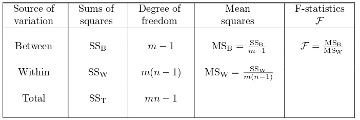
Table 20.1. One-Way ANOVA Table
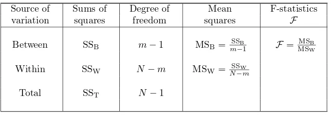
Table 20.2. One-Way ANOVA Table with unequal sample size

Referensi

Dokumen terkait

distribution of the random variables. Analogous to the probability density function of a single continuous random variable, a joint probability density function can be dei ned

A random sample of 280 families with 4 children showed the following number of male and female children as in the given table.. Do the data justify the claim that the probabilities

unreasonable to use probabilities to express how strongly we believe in their truth. It is also obvious that different individuals may assign completely different probabilities.

Use the binomial expansion to find the probabilities of the various combinations of heads and tails... You draw from jars 2 and 4 200 times and get the

Consider two independent events, A and B, with unequal probabilities (i.e. LO.e: Explain the multiplication, addition, and total probability rules. Irfanullah &amp; Co.

One can glean from the two examples above that the sample information is made available to the analyst and, with the aid of statistical methods and elements of probability,

4.84 Referring to the random variables whose joint probability density function is given in Exercise 3.41 on page 105, find the expected weight for the sum of the creams and toffees

 A probability distribution for a discrete random variable is a mutually exclusive listing of all possible numerical outcomes for that variable and a particular probability