Applied Statistics and Probability for E (1)

‡ 6WXGHQWV DFKLHYH FRQFHSW

PDVWHU\ LQ D ULFK

VWUXFWXUHG HQYLURQPHQW

WKDW·V DYDLODEOH

From multiple study paths, to self-assessment, to a wealth of interactive

visual and audio resources,

WileyPLUS

gives you everything you need to

personalize the teaching and learning experience.

:LWK

WileyPLUS

»

)LQG RXW KRZ WR 0$.( ,7 <2856

»

This online teaching and learning environment

integrates the

entire digital textbook

with the

most effective instructor and student resources

WR ÀW HYHU\ OHDUQLQJ VW\OH

‡ ,QVWUXFWRUV SHUVRQDOL]H DQG PDQDJH

WKHLU FRXUVH PRUH HIIHFWLYHO\ ZLWK

DVVHVVPHQW DVVLJQPHQWV JUDGH

WUDFNLQJ DQG PRUH

‡ PDQDJH WLPH EHWWHU

‡ VWXG\ VPDUWHU

‡ VDYH PRQH\

0$.( ,7 <2856

YOU AND YOUR STUDENTS NEED!

7HFKQLFDO 6XSSRUW

)$

4

V RQOLQH FKDW

DQG SKRQH VXSSRUW

www.wileyplus.com/suppor t

6WXGHQW VXSSRUW IURP DQ

H

[

SHULHQFHG VWXGHQW XVHU

$VN \RXU ORFDO UHSUHVHQWDWLYH

IRU GHWDLOV

<RXU

WileyPLUS

$FFRXQW 0DQDJHU

7UDLQLQJ DQG LPSOHPHQWDWLRQ VXSSRUW

www.wileyplus.com/accountmanager

&

ROODERUDWH ZLWK \RXU FROOHDJXHV

ILQG D PHQWRU DWWHQG YLUWXDO DQG OLYH

HYHQWV DQG YLHZ UHVRXUFHV

www.WhereFacultyConnect.com

3

UH

ORDGHG UHDG\

WR

XVH

DVVLJQPHQWV DQG SUHVHQWDWLRQV

www.wiley.com/college/quickstar t

0LQXWH 7XWRULDOV DQG DOO

RI WKH UHVRXUFHV \RX

\RXU

VWXGHQWV QHHG WR JHW VWDUWHG

Applied Statistics

and Probability

for Engineers

Fifth Edition

Douglas C. Montgomery

Arizona State University

George C. Runger

Arizona State University

Meredith, Neil, Colin, and Cheryl

Rebecca, Elisa, George, and Taylor

EXECUTIVE PUBLISHER Don Fowley ASSOCIATE PUBLISHER Daniel Sayre ACQUISITIONS EDITOR Jennifer Welter PRODUCTION EDITOR Trish McFadden MARKETING MANAGER Christopher Ruel SENIOR DESIGNER Kevin Murphy MEDIA EDITOR Lauren Sapira PHOTO ASSOCIATE Sheena Goldstein

EDITORIAL ASSISTANT Alexandra Spicehandler PRODUCTION SERVICES MANAGEMENT Aptara COVER IMAGE Norm Christiansen

This book was set in 10/12 pt. TimesNewRomanPS by Aptara and printed and bound by R.R. Donnelley/ Willard Division. The cover was printed by Phoenix Color.

This book is printed on acid-free paper.

⬁

Copyright © 2011 John Wiley & Sons, Inc. All rights reserved.

No part of this publication may be reproduced, stored in a retrieval system or transmitted in any form or by any means, electronic, mechanical, photocopying, recording, scanning, or otherwise, except as permitted under Sections 107 or 108 of the 1976 United States Copyright Act, without either the prior written permission of the Publisher, or authorization through payment of the appropriate per-copy fee to the Copyright Clearance Center, Inc. 222 Rosewood Drive, Danvers, MA 01923, website www.copyright.com. Requests to the Publisher for permission should be addressed to the Permissions Department, John Wiley & Sons, Inc., 111 River Street, Hoboken, NJ 07030-5774, (201) 748-6011, fax (201) 748-6008, website http://www.wiley.com/go/permissions.

To order books or for customer service, please call 1-800-CALL WILEY (225-5945).

ISBN–13: 978-0-470-05304-1

Printed in the United States of America

Wiley Books by These Authors

Website: www.wiley.com/college/montgomery

Engineering Statistics, Fourth Edition

by Montgomery, Runger, and Hubele

Introduction to engineering statistics, with topical coverage appropriate for a one-semester

course. A modest mathematical level, and an applied approach.

Applied Statistics and Probability for Engineers, Fifth Edition

by Montgomery and Runger

Introduction to engineering statistics, with topical coverage appropriate for either a one- or

two-semester course. An applied approach to solving real-world engineering problems.

Introduction to Statistical Quality Control, Sixth Edition

by Douglas C. Montgomery

For a first course in statistical quality control. A comprehensive treatment of statistical

methodology for quality control and improvement. Some aspects of quality management are

also included, such as the six-sigma approach.

Design and Analysis of Experiments, Seventh Edition

by Douglas C. Montgomery

An introduction to design and analysis of experiments, with the modest prerequisite of a first

course in statistical methods. For senior and graduate students and for practitioners, to design

and analyze experiments for improving the quality and efficiency of working systems.

Introduction to Linear Regression Analysis, Fourth Edition

by Montgomery, Peck, and Vining

A comprehensive and thoroughly up-to-date look at regression analysis, still the most widely used

technique in statistics today.

Response Surface Methodology: Process and Product Optimization Using Designed

Experiments, Third Edition

by Myers, Montgomery, and Anderson-Cook

Website: www.wiley.com/college/myers

The exploration and optimization of response surfaces, for graduate courses in experimental

design, and for applied statisticians, engineers, and chemical and physical scientists.

Generalized Linear Models: With Applications in Engineering and the Sciences

by Myers, Montgomery, and Vining

Website: www.wiley.com/college/myers

An introductory text or reference on generalized linear models (GLMs). The range of theoretical

topics and applications appeals both to students and practicing professionals.

Introduction to Time Series Analysis and Forecasting

by Montgomery, Jennings, and Kulahci

vi

Preface

INTENDED AUDIENCE

This is an introductory textbook for a first course in applied statistics and probability for undergraduate students in engineering and the physical or chemical sciences. These individuals play a significant role in designing and developing new products and manufacturing systems and processes, and they also improve existing systems. Statistical methods are an important tool in these activities because they provide the en-gineer with both descriptive and analytical methods for dealing with the variability in observed data. Although many of the methods we present are fundamental to statistical analysis in other disciplines, such as business and management, the life sciences, and the social sciences, we have elected to focus on an engineering-oriented audience. We believe that this approach will best serve students in engineering and the chemical /physical sciences and will allow them to concentrate on the many applications of statistics in these disciplines. We have worked hard to ensure that our examples and exercises are engineering- and science-based, and in almost all cases we have used examples of real data— either taken from a published source or based on our consulting experiences.

We believe that engineers in all disciplines should take at least one course in statistics. Unfortunately, because of other requirements, most engineers will only take one statistics course. This book can be used for a single course, although we have provided enough material for two courses in the hope that more students will see the important applications of statistics in their everyday work and elect a second course. We believe that this book will also serve as a useful reference.

We have retained the relatively modest mathematical level of the first four editions. We have found that engineering students who have completed one or two semesters of calculus should have no difficulty reading almost all of the text. It is our intent to give the reader an understanding of the methodology and how to apply it, not the mathematical theory. We have made many enhancements in this edition, including reorganizing and rewriting major portions of the book and adding a number of new exercises.

ORGANIZATION OF THE BOOK

Perhaps the most common criticism of engineering statistics texts is that they are too long. Both instructors and students complain that it is impossible to cover all of the topics in the book in one or even two terms. For authors, this is a serious issue because there is great variety in both the content and level of these courses, and the decisions about what material to delete without limiting the value of the text are not easy. Decisions about which topics to include in this edition were made based on a survey of instructors.

Chapter 1 is an introduction to the field of statistics and how engineers use statistical methodology as part of the engineering problem-solving process. This chapter also introduces the reader to some engineer-ing applications of statistics, includengineer-ing buildengineer-ing empirical models, designengineer-ing engineerengineer-ing experiments, and monitoring manufacturing processes. These topics are discussed in more depth in subsequent chapters.

Chapters 2, 3, 4, and 5 cover the basic concepts of probability, discrete and continuous random vari-ables, probability distributions, expected values, joint probability distributions, and independence. We have given a reasonably complete treatment of these topics but have avoided many of the mathematical or more theoretical details.

Chapter 6 begins the treatment of statistical methods with random sampling; data summary and de-scription techniques, including stem-and-leaf plots, histograms, box plots, and probability plotting; and several types of time series plots. Chapter 7 discusses sampling distributions, the central limit theorem, and point estimation of parameters. This chapter also introduces some of the important properties of esti-mators, the method of maximum likelihood, the method of moments, and Bayesian estimation.

PREFACE

vii

the concepts behind them. We give a logical, heuristic development of the procedures rather than a formal, mathematical one. We have also included some material on nonparametric methods in these chapters.

Chapters 11 and 12 present simple and multiple linear regression including model adequacy checking and regression model diagnostics and an introduction to logistic regression. We use matrix algebra throughout the multiple regression material (Chapter 12) because it is the only easy way to understand the concepts presented. Scalar arithmetic presentations of multiple regression are awkward at best, and we have found that undergrad-uate engineers are exposed to enough matrix algebra to understand the presentation of this material.

Chapters 13 and 14 deal with single- and multifactor experiments, respectively. The notions of ran-domization, blocking, factorial designs, interactions, graphical data analysis, and fractional factorials are emphasized. Chapter 15 introduces statistical quality control, emphasizing the control chart and the fun-damentals of statistical process control.

WHAT’S NEW IN THIS EDITION?

We received much feedback from users of the fourth edition of the book, and in response we have made substantial changes in this new edition.

• The most obvious change is that the chapter on nonparametric methods is gone. We have inte-grated most of this material into Chapter 9 and 10 on statistical hypothesis testing, where we think it is a much better fit if instructors elect to cover these techniques.

• Another substantial change is the increased emphasis on the use of P-value in hypothesis test-ing. Many sections of several chapters were rewritten to reflect this.

• We have also rewritten and modified many portions of the book to improve the explanations and try to make the concepts easier to understand.

• We have added brief comments at the end of examples to emphasize the practical interpretations of the results.

• We have also added approximately 200 new homework exercises.

FEATURED IN THIS BOOK

Learning Objectives

Learning Objectives at the start of each chapter guide the students in what they are expected to take away from this chapter and serve as a study reference.

Definitions, Key Concepts, and Equations

Throughout the text, definitions and key con-cepts and equations are highlighted by a box to emphasize their importance.

If Xis a continuous random variable with probability density function f(x),

(4-5) E3h1X2 4⫽冮

⬁

⫺⬁

h1x2f1x2dx Expected

Value of a Function of a Continuous Random Variable

Suppose Xis a continuous random variable with probability density function f(x).

The meanor expected valueof X, denoted as or E(X), is

(4-4)

The varianceof X, denoted as V(X) or is

The standard deviationof Xis ␴ ⫽2␴2. ␴2_⫽V1X2⫽冮

⬁ ⫺⬁

1x⫺ ␮22_f1x2dx⫽冮

⬁ ⫺⬁

x2_{f1x2dx⫺ ␮}2

␴2_,

␮ ⫽E1X2⫽冮 ⬁ ⫺⬁

xf1x2dx

␮

Mean and Variance

4-4 MEAN AND VARIANCE OF A CONTINUOUS RANDOM VARIABLE

The mean and variance can also be defined for a continuous random variable. Integration replaces summation in the discrete definitions. If a probability density function is viewed as a loading on a beam as in Fig. 4-1, the mean is the balance point.

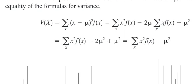
The equivalence of the two formulas for variance can be derived from the same approach used for discrete random variables.

EXAMPLE 4-6 Electric Current

For the copper current measurement in Example 4-1, the mean of Xis

E1X2⫽冮

20 0

xf1x2dx⫽0.05x2_{Ⲑ2 `} 20 0

⫽10

The variance of Xis

V1X2⫽冮

20 0

1x⫺1022_f1x2dx

⫽0.051x⫺1023_{Ⲑ3 `}20 0

⫽33.33

The expected value of a function h(X) of a continuous random variable is also defined in a straightforward manner.

LEARNING OBJECTIVES

After careful study of this chapter you should be able to do the following: 1. Determine probabilities from probability density functions

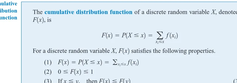
2. Determine probabilities from cumulative distribution functions and cumulative distribution func-tions from probability density funcfunc-tions, and the reverse

3. Calculate means and variances for continuous random variables

4. Understand the assumptions for some common continuous probability distributions 5. Select an appropriate continuous probability distribution to calculate probabilities in specific applications 6. Calculate probabilities, determine means and variances for some common continuous probability

distributions

7. Standardize normal random variables

8. Use the table for the cumulative distribution function of a standard normal distribution to calcu-late probabilities

9-1.6 General Procedure for Hypothesis Tests

This chapter develops hypothesis-testing procedures for many practical problems. Use of the following sequence of steps in applying hypothesis-testing methodology is recommended.

1. Parameter of interest: From the problem context, identify the parameter of interest. 2. Null hypothesis, H0: State the null hypothesis, H0.

3. Alternative hypothesis, H1: Specify an appropriate alternative hypothesis, . 4. Test statistic: Determine an appropriate test statistic.

5. Reject H0if: State the rejection criteria for the null hypothesis.

6. Computations: Compute any necessary sample quantities, substitute these into the equation for the test statistic, and compute that value.

7. Draw conclusions: Decide whether or not H0should be rejected and report that in the problem context.

Steps 1–4 should be completed prior to examination of the sample data. This sequence of steps will be illustrated in subsequent sections.

H1

Figures

Numerous figures throughout the text illustrate statistical concepts in multiple formats.

Seven-Step Procedure for Hypothesis Testing

The text introduces a sequence of seven steps in applying hypothesis-testing methodology and explicitly exhibits this procedure in examples.

Minitab Output

Throughout the book, we have presented output from Minitab as typical examples of what can be done with modern statistical software.

Character Stem-and-Leaf Display Stem-and-leaf of Strength N = 80 Leaf Unit = 1.0

1 7 6

2 8 7

3 9 7

5 10 1 5 8 11 0 5 8 11 12 0 1 3 17 13 1 3 3 4 5 5 25 14 1 2 3 5 6 8 9 9 37 15 0 0 1 3 4 4 6 7 8 8 8 8 (10) 16 0 0 0 3 3 5 7 7 8 9 33 17 0 1 1 2 4 4 5 6 6 8 23 18 0 0 1 1 3 4 6 16 19 0 3 4 6 9 9 10 20 0 1 7 8 6 21 8 5 22 1 8 9 2 23 7 1 24 5

Figure 6-6 A stem-and-leaf diagram from Minitab.

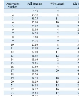
Table 11-1 Oxygen and Hydrocarbon Levels

Observation Hydrocarbon Level Purity

Number x(%) y(%)

1 0.99 90.01

2 1.02 89.05

3 1.15 91.43

4 1.29 93.74

5 1.46 96.73

6 1.36 94.45

7 0.87 87.59

8 1.23 91.77

9 1.55 99.42

10 1.40 93.65

11 1.19 93.54

12 1.15 92.52

13 0.98 90.56

14 1.01 89.54

15 1.11 89.85

16 1.20 90.39

17 1.26 93.25

18 1.32 93.41

19 1.43 94.98

20 0.95 87.33 Figure 11-1 Scatter diagram of oxygen purity versus hydrocarbon level from Table 11-1.

90

88 86

0.95 0.85 92 94 96 98 100

Purity (

y

)

1.05 1.15 1.25 1.35 1.45 1.55 Hydrocarbon level (x)

0 + 1 (1.25)

x = 1.25

x = 1.00

β β

0 + β1 (1.00)

β

True regression line Yx = 0 + 1x

= 75 + 15x

β β µ

y

(Oxygen purity)

x (Hydrocarbon level)

PREFACE

ix

Exercises

Each chapter has an extensive collection of exercises, including end-of-section

exercises that emphasize the material in

that section, supplemental exercises at the end of the chapter that cover the scope of chapter topics and require the student to make a decision about the approach they will use to solve the problem, and mind-expanding

exer-cises that often require the student to

extend the text material somewhat or to apply it in a novel situation.

Answers are provided to most odd-numbered exercises in Appendix C in the text, and the WileyPLUS online learning environment includes for stu-dents complete detailed solutions to selected exercises.

5-67. Suppose that Xis a random variable with probability distribution

Find the probability distribution of Y2X1.

5-68. Let Xbe a binomial random variable with p0.25 and n3. Find the probability distribution of the random variable YX2_.

5-69. Suppose that Xis a continuous random variable with probability distribution

fX1x2

x 18, 0

x6 fX1x214, x1, 2, 3, 4

5-73. Suppose that Xhas the probability distribution

Find the probability distribution of the random variable YeX_.

5-74. The random variable Xhas the probability distri-bution

Find the probability distribution of Y (X 2)2_.

fX1x2

x

8, 0x4 fX1x21, 1x2 EXERCISES FOR SECTION 5-5

(a) Find the probability distribution of the random variable

Y⫽2X⫹10. (b) Find the expected value of Y.

5-70. Suppose that Xhas a uniform probability distribution Show that the probability distribution of the random variable

Y⫽ ⫺2 ln Xis chi-squared with two degrees of freedom.

5-71. A random variable Xhas the following probability distribution:

(a) Find the probability distribution forY⫽X2_.

(b) Find the probability distribution for Y⫽ . (c) Find the probability distribution forY⫽ ln X.

5-72. The velocity of a particle in a gas is a random variable

Vwith probability distribution

where bis a constant that depends on the temperature of the gas and the mass of the particle.

(a) Find the value of the constant a.

(b) The kinetic energy of the particle is . Find the probability distribution of W.

W⫽mV2_Ⲑ2

fV1v2⫽av2e ⫺bv _v⬎0

X1Ⲑ2

fX1x2⫽e ⫺x_{, x}ⱖ0

fX1x2⫽1, 0ⱕxⱕ1 8

Supplemental Exercises

5-75. Show that the following function satisfies the proper-ties of a joint probability mass function:

x y f(x, y)

0 0 1兾4 0 1 1兾8 1 0 1兾8 1 1 1兾4 2 2 1兾4 Determine the following:

(a) (b) (c) (d) (e) Determine E(X), E(Y), V(X), and V(Y).

(f ) Marginal probability distribution of the random vari-able X

(g) Conditional probability distribution of Ygiven that X⫽1 (h)

(i) Are Xand Yindependent? Why or why not? ( j) Calculate the correlation between Xand Y.

5-76. The percentage of people given an antirheumatoid medication who suffer severe, moderate, or minor side effects are 10, 20, and 70%, respectively. Assume that people react

E1Y0X⫽12

P1X⬎0.5, Y⬍1.52 P1X⬍1.52

P1Xⱕ12 P1X⬍0.5, Y⬍1.52

5-96. Show that if X1, X2,p, Xpare independent,

continuous random variables, P(X1僆 A1,X2僆 A2, p , Xp僆 Ap)⫽ P(X1僆 A1)P(X2僆 A2) p P(Xp僆 Ap) for any

regions A1, A2, p , Apin the range of X1, X2, p , Xp

respectively.

5-97. Show that if X1, X2,p, Xpare independent

random variables and Y⫽c1X1⫹ c2X2⫹ ⫹cpXp,

You may assume that the random variables are continuous. 5-98. Suppose that the joint probability function of the continuous random variables Xand Yis constant on the rectangle 0⬍x⬍a, 0⬍y⬍b. Show that Xand Y

are independent.

5-99. Suppose that the range of the continuous variables Xand Yis 0⬍x⬍aand 0⬍y⬍b. Also suppose that the joint probability density function

fXY(x,y)⫽g(x)h(y), where g(x) is a function only of

xand h(y), is a function only of y. Show that Xand Y

are independent.

5-100. This exercise extends the hypergeometric dis-tribution to multiple variables. Consider a population with Nitems of k different types. Assume there are N1

items of type 1, N2items of type 2, ..., Nkitems of type k

so that N1 ⫹N2⫹p⫹p, Nk⫽N. Suppose that a

ran-dom sample of size n is selected, without replacement, from the population. Let X1, X2, ..., Xkdenote the number of items of each type in the sample so that X1, X2, ⫹p⫹ p, Xk⫽n. Show that for feasible values of the

parame-ters n, x1, x2, p, xk, N1, N2, p, Nk, the probability is P(X1⫽

x1, X2⫽x2, p, Xk⫽xk) ⫽

aN1_x1baN2_x2bpa Nk xnb

aN nb V1Y2⫽c2_1V1X12

⫹c2_2V1X22

⫹p⫹c2_pV1Xp2 p

MIND-EXPANDING EXERCISES

IMPORTANT TERMS AND CONCEPTS

Bivariate distribution Bivariate normal

distribution Conditional mean

Multinomial distribution Reproductive property of

the normal distribution Conditional variance Contour plots Correlation Covariance

Joint probability density function Joint probability mass

function

Important Terms and Concepts

At the end of each chapter is a list of important terms and concepts for an easy self-check and study tool.

STUDENT RESOURCES

• Data Sets Data sets for all examples and exercises in the text. Visit the student section of the book Web site at www.wiley.com /college/montgomery to access these materials.

• Student Solutions Manual Detailed solutions for selected problems in the book. The Student

Solutions Manual may be purchased from the Web site at www.wiley.com /college/montgomery. Example Problems

A set of example problems provides the stu-dent with detailed solutions and comments for interesting, real-world situations. Brief practi-cal interpretations have been added in this edition.

EXAMPLE 10-1 Paint Drying Time

A product developer is interested in reducing the drying time of a primer paint. Two formulations of the paint are tested; for-mulation 1 is the standard chemistry, and forfor-mulation 2 has a new drying ingredient that should reduce the drying time. From experience, it is known that the standard deviation of drying time is 8 minutes, and this inherent variability should be unaffected by the addition of the new ingredient. Ten spec-imens are painted with formulation 1, and another 10 speci-mens are painted with formulation 2; the 20 specispeci-mens are painted in random order. The two sample average drying times are minutes and minutes, respectively. What conclusions can the product developer draw about the effectiveness of the new ingredient, using ␣ ⫽0.05?

We apply the seven-step procedure to this problem as follows:

1. Parameter of interest:The quantity of interest is the dif-ference in mean drying times, ␮1⫺ ␮2, and ⌬0⫽0. 2. Non hypothesis:

3. Alternative hypothesis: We want to reject

H₀if the new ingredient reduces mean drying time.

H˛1: ␮1⬎ ␮2. H˛₀: ␮₁⫺ ␮₂⫽0, or H˛₀:˛␮₁⫽ ␮₂.

x˛₂⫽112 x˛₁⫽121

4. Test statistic:The test statistic is

where ␴2

1⫽ ␴22⫽ ⫽64 and n1⫽n2⫽10. 5. Reject H0if:Reject H0: ␮1⫽ ␮2if the P-value is less

than 0.05.

6. Computations:Since minutes and

minutes, the test statistic is

7. Conclusion:Since z

0⫽2.52, the P-value is P⫽

, so we reject H₀at the ␣ ⫽0.05 level Practical Interpretation: We conclude that adding the new ingredient to the paint significantly reduces the drying time. This is a strong conclusion.

1⫺ ⌽12.522⫽0.0059

z₀⫽ 121⫺112 B1

822

10⫹

1822

10 ⫽2.52

x₂⫽112

x₁⫽121

1822 z˛₀⫽

x₁⫺x₂⫺0

B ␴2

1 n₁⫹

INSTRUCTOR RESOURCES

The following resources are available only to instructors who adopt the text:

• Solutions Manual All solutions to the exercises in the text.

• Data Sets Data sets for all examples and exercises in the text.

• Image Gallery of Text Figures

• PowerPoint Lecture Slides

• Section on Logistic Regression

These instructor-only resources are password-protected. Visit the instructor section of the book Web site at www.wiley.com /college/montgomery to register for a password to access these materials.

MINITAB

A student version of Minitab is available as an option to purchase in a set with this text. Student versions of software often do not have all the functionality that full versions do. Consequently, student versions may not support all the concepts presented in this text. If you would like to adopt for your course the set of this text with the student version of Minitab, please contact your local Wiley representative at www.wiley.com/college/rep.

Alternatively, students may find information about how to purchase the professional version of the software for academic use at www.minitab.com.

WileyPLUS

This online teaching and learning environment integrates the entire digital textbook with the most effective instructor and student resources to fit every learning style.

With WileyPLUS:

• Students achieve concept mastery in a rich, structured environment that’s available 24/7. • Instructors personalize and manage their course more effectively with assessment, assignments,

grade tracking, and more.

WileyPLUS can complement your current textbook or replace the printed text altogether.

For Students

Personalize the learning experience

Different learning styles, different levels of proficiency, different levels of preparation—each of your stu-dents is unique. WileyPLUS empowers them to take advantage of their individual strengths:

• Students receive timely access to resources that address their demonstrated needs, and get im-mediate feedback and remediation when needed.

• Integrated, multi-media resources—including audio and visual exhibits, demonstration prob-lems, and much more—provide multiple study-paths to fit each student’s learning preferences and encourage more active learning.

• WileyPLUS includes many opportunities for self-assessment linked to the relevant portions

PREFACE

xi

For Instructors

Personalize the teaching experience

WileyPLUS empowers you with the tools and resources you need to make your teaching even more

effective:

• You can customize your classroom presentation with a wealth of resources and functionality from PowerPoint slides to a database of rich visuals. You can even add your own materials to your WileyPLUS course.

• With WileyPLUS you can identify those students who are falling behind and intervene accord-ingly, without having to wait for them to come to office hours.

• WileyPLUS simplifies and automates such tasks as student performance assessment, making

as-signments, scoring student work, keeping grades, and more.

COURSE SYLLABUS SUGGESTIONS

This is a very flexible textbook because instructors’ ideas about what should be in a first course on sta-tistics for engineers vary widely, as do the abilities of different groups of students. Therefore, we hesitate to give too much advice, but will explain how we use the book.

We believe that a first course in statistics for engineers should be primarily an applied statistics course, not a probability course. In our one-semester course we cover all of Chapter 1 (in one or two lectures); overview the material on probability, putting most of the emphasis on the normal distribution (six to eight lectures); discuss most of Chapters 6 through 10 on confidence intervals and tests (twelve to fourteen lectures); introduce regression models in Chapter 11 (four lectures); give an introduction to the design of experiments from Chapters 13 and 14 (six lectures); and present the basic concepts of statisti-cal process control, including the Shewhart control chart from Chapter 15 (four lectures). This leaves about three to four periods for exams and review. Let us emphasize that the purpose of this course is to introduce engineers to how statistics can be used to solve real-world engineering problems, not to weed out the less mathematically gifted students. This course is not the “baby math-stat” course that is all too often given to engineers.

If a second semester is available, it is possible to cover the entire book, including much of the supplemental material, if appropriate for the audience. It would also be possible to assign and work many of the homework problems in class to reinforce the understanding of the concepts. Obviously, multiple regression and more design of experiments would be major topics in a second course.

USING THE COMPUTER

In practice, engineers use computers to apply statistical methods to solve problems. Therefore, we strongly recommend that the computer be integrated into the class. Throughout the book we have presented output from Minitab as typical examples of what can be done with modern statistical software. In teaching, we have used other software packages, including Statgraphics, JMP, and Statistica. We did not clutter up the book with examples from many different packages because how the instructor integrates the software into the class is ultimately more important than which package is used. All text data are available in electronic form on the textbook Web site. In some chapters, there are problems that we feel should be worked using computer software. We have marked these problems with a special icon in the margin.

Users should be aware that final answers may differ slightly due to different numerical precision and rounding protocols among softwares.

ACKNOWLEDGMENTS

We would like to express our grateful appreciation to the many organizations and individuals who have contributed to this book. Many instructors who used the previous editions provided excellent suggestions that we have tried to incorporate in this revision.

We would like to thank the following who assisted in contributing to and/or reviewing material for the WileyPLUS course:

Michael DeVasher, Rose-Hulman Institute of Technology Craig Downing, Rose-Hulman Institute of Technology Julie Fortune, University of Alabama in Huntsville Rubin Wei, Texas A&M University

We would also like to thank the following for their assistance in checking the accuracy and com-pleteness of the exercises and the solutions to exercises.

Abdelaziz Berrado, Arizona State University Dr. Connie Borror, Arizona State Universtity Patrick Egbunonu, Queens University James C. Ford, Ford Consulting Associates Dr. Alejandro Heredia-Langner

Jing Hu, Arizona State University

Busaba Laungrungrong, Arizona State University Fang Li, Arizona State University

Nuttha Lurponglukana, Arizona State University Sarah Streett

Yolande Tra, Rochester Institute of Technology Dr. Lora Zimmer

We are also indebted to Dr. Smiley Cheng for permission to adapt many of the statistical tables from his excellent book (with Dr. James Fu), Statistical Tables for Classroom and Exam Room. John Wiley and Sons, Prentice Hall, the Institute of Mathematical Statistics, and the editors of Biometrics allowed us to use copyrighted material, for which we are grateful.

Contents

xiii

INSIDE FRONT COVER

Index of Applications in

Examples and Exercises

CHAPTER 1

The Role of Statistics in Engineering 1

1-1 The Engineering Method and Statistical Thinking 2

1-2 Collecting Engineering Data 5

1-2.1 Basic Principles 5 1-2.2 Retrospective Study 5 1-2.3 Observational Study 6 1-2.4 Designed Experiments 6 1-2.5 Observing Processes Over Time 9

1-3 Mechanistic and Empirical Models 12

1-4 Probability and Probability Models 15

CHAPTER 2

Probability

17

2-1 Sample Spaces and Events 18

2-1.1 Random Experiments 18 2-1.2 Sample Spaces 19 2-1.3 Events 22

2-1.4 Counting Techniques 24

2-2 Interpreta

tions and Axioms of Proba

bility 31

2-3 Addition Rules 37

2-4 Conditional Probability 41

2-5 Multiplication and Total Probability Rules 47

2-6 Independence 50

2-7 Bayes’ Theorem 55

2-8 Random Variables 57

CHAPTER 3

Discrete Random Variables and

Probability Distributions

66

3-1 Discrete Random Variables 67

3-2 Probability Distributions and Probability Mass

Functions 68

3-3 Cumulative Distribution Functions 71

3-4 Mean and Variance of a Discrete Random Variable 74

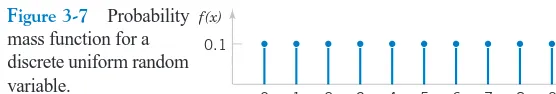
3-5 Discrete Uniform Distribution 77

3-6 Binomial Distribution 79

3-7 Geometric and Negative Binomial Distributions 86

3-8 Hypergeometric Distribution 92

3-9 Poisson Distribution 97

CHAPTER 4

Continuous Random Variables and

Probability Distributions

107

4-1 Continuous Random Variables 108

4-2 Probability Distributions and Probability Density

Functions 108

4-3 Cumulative Distribution Functions 111

4-4 Mean and Variance of a Continuous Random

Variable 114

4-5 Continuous Uniform Distribution 116

4-6 Normal Distribution 118

4-7 Normal Approximation to the Binomial and Poisson Distributions 127

4-8 Exponential Distribution 132

4-9 Erlang and Gamma Distributions 138

4-10 Weibull Distribution 141

4-11 Lognormal Distribution 144

4-12 Beta Distribution 146

CHAPTER 5

Joint Probability Distributions

152

5-1 Two or More Random Variables 153

5-1.1 Joint Probability Distributions 153 5-1.2 Marginal Probability Distributions 156 5-1.3 Conditional Probability Distributions 158 5-1.4 Independence 161

5-1.5 More Than Two Random Variables 163

5-2 Covariance and Correlation 170

5-3 Common Joint Distributions 176

5-3.1 Multinomial Distribution 176 5-3.2 Bivariate Normal Distribution 177

5-4 Linear Functions of Random Variables 181

5-5 General Functions of Random Variables 185

CHAPTER 6

Descriptive Statistics

191

6-1 Numerical Summaries of Data 192

6-2 Stem-and-Leaf Diagrams 197

6-3 Frequency Distributions and Histograms 203

6-4 Box Plots 208

6-5 Time Sequence Plots 210

6-6 Probability Plots 214

CHAPTER 7

Sampling Distributions and Point

Estimation of Parameters

223

7-1 Point Estimation 224

7-2 Sampling Distributions and the Central Limit

Theorem 225

7-3 General Concepts of Point Estimation 231

7-3.1 Unbiased Estimators 231 7-3.2 Variance of a Point Estimator 232

7-3.3 Standard Error: Reporting a Point Estimate 233 7-3.4 Mean Squared Error of an Estimator 234

7-4 Methods of Point Estimation 237

7-4.1 Method of Moments 237

7-4.2 Method of Maximum Likelihood 239 7-4.3 Bayesian Estimation of Parameters 244

CHAPTER 8

Statistical Intervals for a Single

Sample

251

8-1 Confidence Interval on the Mean of a Normal Distribution, Variance Known 253

8-1.1 Development of the Confidence Interval and Its Basic Properties 253

8-1.2 Choice of Sample Size 256 8-1.3 One-sided Confidence Bounds 257 8-1.4 General Method to Derive a

Confidence Interval 258

8-1.5 Large-Sample Confidence Interval for ␮ 258

8-2 Confidence Interval on the Mean of a Normal Distribution, Variance Unknown 261

8-2.1 tDistribution 262

8-3 Confidence Interval on the Variance and Standard Deviation of a Normal Distribution 266

8-4 Large-Sample Confidence Interval for a Population

Proportion 270

8-5 Guidelines for Constructing Confidence Intervals 273 8-6 Tolerance and Prediction Intervals 274

8-6.1 Prediction Interval for a Future Observation 274 8-6.2 Tolerance Interval for a Normal Distribution 276

CHAPTER 9

Tests of Hypotheses for a Single

Sample

283

9-1 Hypothesis Testing 284

9-1.1 Statistical Hypotheses 284 9-1.2 Tests of Statistical Hypotheses 286 9-1.3 One-Sided and Two-Sided Hypothesis 292 9-1.4 P-Values in Hypothesis Tests 294 9-1.5 Connection between Hypothesis Tests and

Confidence Intervals 295

9-1.6 General Procedure for Hypothesis Tests 296

9-2 Tests on the Mean of a Normal Distribution, Variance

Known 299

9-2.1 Hypothesis Tests on the Mean 299 9-2.2 Type II Error and Choice of Sample Size 303 9-2.3 Large-Sample Test 307

9-3 Tests on the Mean of a Normal Distribution, Variance

Unknown 310

9-3.1 Hypothesis Tests on the Mean 310 9-3.2 Type II Error and Choice of Sample Size 314

9-4 Tests on the Variance and Standard Deviation of a Normal Distribution 319

9-4.1 Hypothesis Tests on the Variance 319 9-4.2 Type II Error and Choice of Sample Size 322

9-5 Tests on a Population Proportion 323

9-5.1 Large-Sample Tests on a Proportion 324 9-5.2 Type II Error and Choice of Sample Size 326

9-6 Summary Table of Inference Procedures for a Single

Sample 329

9-7 Testing for Goodness of Fit 330

9-8 Contingency Table Tests 333

9-9 Nonparametric Procedures 337

9-9.1 The Sign Test 337

9-9.2 The Wilcoxon Signed-Rank Test 342 9-9.3 Comparison to the t-Test 344

CHAPTER 10

Statistical Inference for Two

Samples

351

10-1 Inference on the Difference in Means of Two Normal Distributions, Variances Known 352

10-1.1 Hypothesis Tests on the Difference in Means, Variances Known 354

10-1.2 Type II Error and Choice of Sample Size 356 10-1.3 Confidence Interval on the Difference in Means,

Variances Known 357

10-2 Inference on the Difference in Means of Two Normal Distributions, Variances Unknown 361

10-2.1 Hypothesis Tests on the Difference in Means, Variances Unknown 361

10-2.2 Type II Error and Choice of Sample Size 367 10-2.3 Confidence Interval on the Difference in Means,

Variances Unknown 368

10-3 A Nonparametric Test for the Difference in Two

Means 373

10-3.1 Description of the Wilcoxon Rank-Sum Test 373 10-3.2 Large-Sample Approximation 374

10-3.3 Comparison to the t-Test 375

10-4 Paired t-Test 376

10-5 Inference on the Variances of Two Normal Distributions 382

10-5.1 FDistribution 383

10-5.2 Hypothesis Tests on the Ratio of Two Variances 384 10-5.3 Type II Error and Choice of Sample Size 387 10-5.4 Confidence Interval on the Ratio of Two

Variances 387

10-6 Inference on Two Population Proportions 389

10-6.1 Large-Sample Tests on the Difference in Population Proportions 389

10-6.2 Type II Error and Choice of Sample Size 391 10-6.3 Confidence Interval on the Difference in Population

Proportions 392

10-7 Summary Table and Roadmap for Inference Procedures for Two Samples 394

CHAPTER 11

Simple Linear Regression and

Correlation

401

11-1 Empirical Models 402

11-2 Simple Linear Regression 405

11-3 Properties of the Least Squares Estimators 414 11-4 Hypothesis Tests in Simple Linear Regression 415

11-4.1 Use of t-Tests 415

11-4.2 Analysis of Variance Approach to Test Significance of Regression 417

11-5 Confidence Intervals 421

11-5.1 Confidence Intervals on the Slope and Intercept 421 11-5.2 Confidence Interval on the Mean Response 421

11-6 Prediction of New Observations 423

11-7 Adequacy of the Regression Model 426

11-7.1 Residual Analysis 426

11-7.2 Coefficient of Determination (R2_{) 428}

11-8 Correlation 431

11-9 Regression on Transformed Variables 437

11-10 Logistic Regression 440

CHAPTER 12

Multiple Linear Regression

449

12-1 Multiple Linear Regression Model 450

12-1.1 Introduction 450

12-1.2 Least Squares Estimation of the Parameters 452 12-1.3 Matrix Approach to Multiple Linear Regression 456 12-1.4 Properties of the Least Squares Estimators 460

12-2 Hypothesis Tests in Multiple Linear Regression 470

12-2.1 Test for Significance of Regression 470 12-2.2 Tests on Individual Regression Coefficients and

Subsets of Coefficients 472

12-3 Confidence Intervals in Multiple Linear Regression 479

12-3.1 Confidence Intervals on Individual Regression Coefficients 479

12-3.2 Confidence Interval on the Mean Response 480

12-4 Prediction of New Observations 481

12-5 Model Adequacy Checking 484

CONTENTS

xv

12-6 Aspects of Multiple Regression Modeling 490

12-6.1 Polynomial Regression Models 490

12-6.2 Categorical Regressors and Indicator Variables 492 12-6.3 Selection of Variables and Model Building 494 12-6.4 Multicollinearity 502

CHAPTER 13

Design and Analysis of Single-Factor

Experiments: The Analysis of Variance

513

13-1 Designing Engineering Experiments 514

13-2 Completely Randomized Single-Factor

Experiment 515

13-2.1 Example: Tensile Strength 515 13-2.2 Analysis of Variance 517

13-2.3 Multiple Comparisons Following the ANOVA 524 13-2.4 Residual Analysis and Model Checking 526 13-2.5 Determining Sample Size 527

13-3 The Random-Effects Model 533

13-3.1 Fixed Versus Random Factors 533 13-3.2 ANOVA and Variance Components 534

13-4 Randomized Complete Block Design 538

13-4.1 Design and Statistical Analysis 538 13-4.2 Multiple Comparisons 542

13-4.3 Residual Analysis and Model Checking 544

CHAPTER 14

Design of Experiments with

Several Factors

551

14-1 Introduction 552

14-2 Factorial Experiments 555

14-3 Two-Factor Factorial Experiments 558

14-3.1 Statistical Analysis of the Fixed-Effects Model 559 14-3.2 Model Adequacy Checking 564

14-3.3 One Observation per Cell 566

14-4 General Factorial Experiments 568 14-5 2k_{Factorial Designs 571}

14-5.1 22_{Design 571}

14-5.2 2k_{Design for k}

ⱖ3 Factors 577 14-5.3 Single Replicate of the 2k_{Design 584}

14-5.4 Addition of Center Points to a 2k_{Design 588} 14-6 Blocking and Confounding in the 2k_{Design 595} 14-7 Fractional Replication of the 2k_{Design 602}

14-7.1 One-Half Fraction of the 2k_{Design 602}

14-7.2 Smaller Fractions: The 2k⫺p_Fractional

Factorial 608

14-8 Response Surface Methods and Designs 619

CHAPTER 15

Statistical Quality Control

637

15-1 Quality Improvement and Statistics 638

15-1.1 Statistical Quality Control 639 15-1.2 Statistical Process Control 640

15-2 Introduction to Control Charts 640

15-2.1 Basic Principles 640

15-2.2 Design of a Control Chart 644

15-2.3 Rational Subgroups 646

15-2.4 Analysis of Patterns on Control Charts 647

15-3 and Ror SControl Charts 649

15-4 Control Charts for Individual Measurements 658 15-5 Process Capability 662

15-6 Attribute Control Charts 668

15-6.1 PChart (Control Chart for Proportions) 668 15-6.2 UChart (Control Chart for Defects per Unit) 670

15-7 Control Chart Performance 673

15-8 Time-Weighted Charts 676

15-8.1 Cumulative Sum Control Chart 676

15-8.2 Exponentially Weighted Moving Average Control Chart 682

15-9 Other SPC Problem-Solving Tools 688

15-10 Implementing SPC 690

APPENDICES

702

APPENDIX A:

Statistical Tables and Charts

703

Table I Summary of Common Probability

Distributions 704

Table II Cumulative Binomial Probability

P(X x) 705

Table III Cumulative Standard Normal Distribution 708 Table IV Percentage Points ␹2␣,␯of the Chi-Squared

Distribution 710

Table V Percentage Points t␣,␯of the tdistribution 711 Table VI Percentage Points f␣,v1,v2of the Fdistribution 712 Chart VII Operating Characteristic Curves 717

Table VIII Critical Values for the Sign Test 726 Table IX Critical Values for the Wilcoxon Signed-Rank

Test 726

Table X Critical Values for the Wilcoxon Rank-Sum

Test 727

Table XI Factors for Constructing Variables Control

Charts 728

Table XII Factors for Tolerance Intervals 729

APPENDIX B:

Answers to Selected Exercises

731

APPENDIX C:

Bibliography

749

GLOSSARY

751

INDEX

762

INDEX OF APPLICATIONS IN EXAMPLES

AND EXERCISES, CONTINUED

766

ⱕ

1

1

©Steve Shepard/iStockphoto

The Role of Statistics

in Engineering

Statistics is a science that helps us make decisions and draw conclusions in the

pres-ence of variability. For example, civil engineers working in the transportation field are

concerned about the capacity of regional highway systems. A typical problem would

involve data on the number of nonwork, home-based trips, the number of persons per

household, and the number of vehicles per household, and the objective would be to

produce a trip-generation model relating trips to the number of persons per household

and the number of vehicles per household. A statistical technique called regression

analysis can be used to construct this model. The trip-generation model is an important

tool for transportation systems planning. Regression methods are among the most

widely used statistical techniques in engineering. They are presented in Chapters 11

and 12.

CHAPTER OUTLINE

LEARNING OBJECTIVES

After careful study of this chapter you should be able to do the following:

1. Identify the role that statistics can play in the engineering problem-solving process

2. Discuss how variability affects the data collected and used for making engineering decisions 3. Explain the difference between enumerative and analytical studies

4. Discuss the different methods that engineers use to collect data

5. Identify the advantages that designed experiments have in comparison to other methods of collecting engineering data

6. Explain the differences between mechanistic models and empirical models

7. Discuss how probability and probability models are used in engineering and science

1-1

THE ENGINEERING METHOD AND STATISTICAL THINKING

An engineer is someone who solves problems of interest to society by the efficient application

of scientific principles. Engineers accomplish this by either refining an existing product or

process or by designing a new product or process that meets customers’ needs. The engineering,

or scientific, method is the approach to formulating and solving these problems. The steps in

the engineering method are as follows:

1.

Develop a clear and concise description of the problem.

2.

Identify, at least tentatively, the important factors that affect this problem or that may

play a role in its solution.

3.

Propose a model for the problem, using scientific or engineering knowledge of the

phenomenon being studied. State any limitations or assumptions of the model.

4.

Conduct appropriate experiments and collect data to test or validate the tentative

model or conclusions made in steps 2 and 3.

5.

Refine the model on the basis of the observed data.

1-1 THE ENGINEERING METHOD AND STATISTICAL THINKING

1-2 COLLECTING ENGINEERING DATA

1-2.1 Basic Principles

1-2.2 Retrospective Study

1-2.3 Observational Study

1-2.4 Designed Experiments

1-2.5 Observing Processes Over Time

1-3 MECHANISTIC AND EMPIRICAL MODELS

1-4 PROBABILITY AND PROBABILITY MODELS

1-1 THE ENGINEERING METHOD AND STATISTICAL THINKING

3

Figure 1-1 The engineering method.

Develop a clear description

Identify the important

factors

Propose or refine a

model

Conduct experiments

Manipulate the model

Confirm the solution

Conclusions and recommendations

6.

Manipulate the model to assist in developing a solution to the problem.

7.

Conduct an appropriate experiment to confirm that the proposed solution to the

problem is both effective and efficient.

8.

Draw conclusions or make recommendations based on the problem solution.

The steps in the engineering method are shown in Fig. 1-1. Many of the engineering sciences

are employed in the engineering method: the mechanical sciences (statics, dynamics), fluid

science, thermal science, electrical science, and the science of materials. Notice that the

engi-neering method features a strong interplay between the problem, the factors that may influence

its solution, a model of the phenomenon, and experimentation to verify the adequacy of the

model and the proposed solution to the problem. Steps 2–4 in Fig. 1-1 are enclosed in a box,

indicating that several cycles or iterations of these steps may be required to obtain the final

solution. Consequently, engineers must know how to efficiently plan experiments, collect data,

analyze and interpret the data, and understand how the observed data are related to the model

they have proposed for the problem under study.

The field of

statistics

deals with the collection, presentation, analysis, and use of data to

make decisions, solve problems, and design products and processes. In simple terms, statistics

is the science of data. Because many aspects of engineering practice involve working with

data, obviously knowledge of statistics is just as important to an engineer as the other engineering

sciences. Specifically, statistical techniques can be a powerful aid in designing new products

and systems, improving existing designs, and designing, developing, and improving production

processes.

Statistical methods are used to help us describe and understand variability. By variability,

we mean that successive observations of a system or phenomenon do not produce exactly the

same result. We all encounter variability in our everyday lives, and statistical thinking can

give us a useful way to incorporate this variability into our decision-making processes. For

example, consider the gasoline mileage performance of your car. Do you always get exactly the

same mileage performance on every tank of fuel? Of course not—in fact, sometimes the mileage

performance varies considerably. This observed variability in gasoline mileage depends on

many factors, such as the type of driving that has occurred most recently (city versus

high-way), the changes in condition of the vehicle over time (which could include factors such as

tire inflation, engine compression, or valve wear), the brand and /or octane number of the

gasoline used, or possibly even the weather conditions that have been recently experienced.

These factors represent potential sources of variability in the system. Statistics provides a

framework for describing this variability and for learning about which potential sources of

variability are the most important or which have the greatest impact on the gasoline mileage

performance.

at 3

兾

32 inch but is somewhat uncertain about the effect of this decision on the connector

pull-off force. If the pull-pull-off force is too low, the connector may fail when it is installed in an

en-gine. Eight prototype units are produced and their pull-off forces measured, resulting in the

following data (in pounds): 12.6, 12.9, 13.4, 12.3, 13.6, 13.5, 12.6, 13.1. As we anticipated,

not all of the prototypes have the same pull-off force. We say that there is variability in the

pull-off force measurements. Because the pull-off force measurements exhibit variability, we

consider the pull-off force to be a

random variable.

A convenient way to think of a random

variable, say X, that represents a measurement is by using the model

(1-1)

where

␮

is a constant and

⑀

is a random disturbance. The constant remains the same with every

measurement, but small changes in the environment, variance in test equipment, differences in

the individual parts themselves, and so forth change the value of

⑀

. If there were no

distur-bances,

⑀

would always equal zero and X would always be equal to the constant

␮

. However,

this never happens in the real world, so the actual measurements X exhibit variability. We often

need to describe, quantify, and ultimately reduce variability.

Figure 1-2 presents a dot diagram of these data. The dot diagram is a very useful plot for

displaying a small body of data—say, up to about 20 observations. This plot allows us to see

easily two features of the data: the location, or the middle, and the scatter or variability. When

the number of observations is small, it is usually difficult to identify any specific patterns in the

variability, although the dot diagram is a convenient way to see any unusual data features.

The need for statistical thinking arises often in the solution of engineering problems.

Consider the engineer designing the connector. From testing the prototypes, he knows that the

average pull-off force is 13.0 pounds. However, he thinks that this may be too low for the

intended application, so he decides to consider an alternative design with a greater wall

thickness, 1

兾

8 inch. Eight prototypes of this design are built, and the observed pull-off force

measurements are 12.9, 13.7, 12.8, 13.9, 14.2, 13.2, 13.5, and 13.1. The average is 13.4.

Results for both samples are plotted as dot diagrams in Fig. 1-3. This display gives the

im-pression that increasing the wall thickness has led to an increase in pull-off force. However,

there are some obvious questions to ask. For instance, how do we know that another sample

of prototypes will not give different results? Is a sample of eight prototypes adequate to give

reliable results? If we use the test results obtained so far to conclude that increasing the wall

thickness increases the strength, what risks are associated with this decision? For example,

is it possible that the apparent increase in pull-off force observed in the thicker prototypes

is only due to the inherent variability in the system and that increasing the thickness of the

part (and its cost) really has no effect on the pull-off force?

Often, physical laws (such as Ohm’s law and the ideal gas law) are applied to help design

products and processes. We are familiar with this reasoning from general laws to specific

cases. But it is also important to reason from a specific set of measurements to more general

cases to answer the previous questions. This reasoning is from a

sample

(such as the eight

connectors) to a

population

(such as the connectors that will be sold to customers). The

reasoning is referred to as statistical inference. See Fig. 1-4. Historically, measurements were

X

⫽ ␮ ⫹ ⑀

12 13 14 15

Pull-off force

Figure 1-2 Dot diagram of the pull-off force data when wall thickness is 3/32 inch.

12 13 14 15

Pull-off force

3 32inch

inch

=

1 8 =

1-2 COLLECTING ENGINEERING DATA

5

Physical laws

Types of reasoning

Product designs

Population

Statistical inference

Sample Figure 1-4 Statistical

inference is one type of reasoning.

obtained from a sample of people and generalized to a population, and the terminology has

remained. Clearly, reasoning based on measurements from some objects to measurements on

all objects can result in errors (called sampling errors). However, if the sample is selected

properly, these risks can be quantified and an appropriate sample size can be determined.

1-2

COLLECTING ENGINEERING DATA

1-2.1

Basic Principles

In the previous section, we illustrated some simple methods for summarizing data. Sometimes

the data are all of the observations in the populations. This results in a census. However, in the

engineering environment, the data are almost always a sample that has been selected from the

population. Three basic methods of collecting data are

A retrospective study using historical data

An observational study

A designed experiment

An effective data-collection procedure can greatly simplify the analysis and lead to improved

understanding of the population or process that is being studied. We now consider some

examples of these data-collection methods.

1-2.2

Retrospective Study

Montgomery, Peck, and Vining (2006) describe an acetone-butyl alcohol distillation column

for which concentration of acetone in the distillate or output product stream is an important

variable. Factors that may affect the distillate are the reboil temperature, the condensate

tem-perature, and the reflux rate. Production personnel obtain and archive the following records:

The concentration of acetone in an hourly test sample of output product

The reboil temperature log, which is a plot of the reboil temperature over time

The condenser temperature controller log

The nominal reflux rate each hour

The reflux rate should be held constant for this process. Consequently, production personnel

change this very infrequently.

among the two temperatures and the reflux rate on the acetone concentration in the output

product stream. However, this type of study presents some problems:

1.

We may not be able to see the relationship between the reflux rate and acetone

con-centration, because the reflux rate didn’t change much over the historical period.

2.

The archived data on the two temperatures (which are recorded almost continuously)

do not correspond perfectly to the acetone concentration measurements (which are

made hourly). It may not be obvious how to construct an approximate correspondence.

3.

Production maintains the two temperatures as closely as possible to desired targets or

set points. Because the temperatures change so little, it may be difficult to assess their

real impact on acetone concentration.

4.

In the narrow ranges within which they do vary, the condensate temperature tends to

increase with the reboil temperature. Consequently, the effects of these two process

variables on acetone concentration may be difficult to separate.

As you can see, a retrospective study may involve a lot of data, but those data may contain

relatively little useful information about the problem. Furthermore, some of the relevant

data may be missing, there may be transcription or recording errors resulting in

outliers

(or unusual values), or data on other important factors may not have been collected and

archived. In the distillation column, for example, the specific concentrations of butyl alcohol

and acetone in the input feed stream are a very important factor, but they are not archived

because the concentrations are too hard to obtain on a routine basis. As a result of these types

of issues, statistical analysis of historical data sometimes identifies interesting phenomena,

but solid and reliable explanations of these phenomena are often difficult to obtain.

1-2.3

Observational Study

In an observational study, the engineer observes the process or population, disturbing it as

little as possible, and records the quantities of interest. Because these studies are usually

con-ducted for a relatively short time period, sometimes variables that are not routinely measured

can be included. In the distillation column, the engineer would design a form to record the two

temperatures and the reflux rate when acetone concentration measurements are made. It may

even be possible to measure the input feed stream concentrations so that the impact of this

factor could be studied. Generally, an observational study tends to solve problems 1 and 2

above and goes a long way toward obtaining accurate and reliable data. However,

observa-tional studies may not help resolve problems 3 and 4.

1-2.4

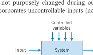
Designed Experiments

In a designed experiment the engineer makes deliberate or purposeful changes in the

control-lable variables of the system or process, observes the resulting system output data, and then

makes an inference or decision about which variables are responsible for the observed changes

in output performance. The nylon connector example in Section 1-1 illustrates a designed

experiment; that is, a deliberate change was made in the wall thickness of the connector with

the objective of discovering whether or not a greater pull-off force could be obtained.

Experiments designed with basic principles such as randomization are needed to establish

cause-and-effect relationships.

1-2 COLLECTING ENGINEERING DATA

7

Table 1-1 The Designed Experiment (Factorial Design) for the Distillation Column

Reboil Temp. Condensate Temp. Reflux Rate

⫺1 ⫺1 ⫺1

⫹1 ⫺1 ⫺1

⫺1 ⫹1 ⫺1

⫹1 ⫹1 ⫺1

⫺1 ⫺1 ⫹1

⫹1 ⫺1 ⫹1

⫺1 ⫹1 ⫹1

⫹1 ⫹1 ⫹1

scientific or engineering theory is directly or completely applicable, so experimentation and

observation of the resulting data constitute the only way that the problem can be solved. Even

when there is a good underlying scientific theory that we may rely on to explain the

phenom-ena of interest, it is almost always necessary to conduct tests or experiments to confirm that the

theory is indeed operative in the situation or environment in which it is being applied.

Statistical thinking and statistical methods play an important role in planning, conducting, and

analyzing the data from engineering experiments. Designed experiments play a very important

role in engineering design and development and in the improvement of manufacturing processes.

For example, consider the problem involving the choice of wall thickness for the

nylon connector. This is a simple illustration of a designed experiment. The engineer chose two

wall thicknesses for the connector and performed a series of tests to obtain pull-off force

measurements at each wall thickness. In this simple comparative experiment, the engineer is

interested in determining if there is any difference between the 3

兾

32- and 1

兾

8-inch designs. An

approach that could be used in analyzing the data from this experiment is to compare the mean

pull-off force for the 3

兾

32-inch design to the mean pull-off force for the 1

兾

8-inch design using

statistical

hypothesis testing,

which is discussed in detail in Chapters 9 and 10. Generally, a

hypothesis

is a statement about some aspect of the system in which we are interested. For

example, the engineer might want to know if the mean pull-off force of a 3

兾

32-inch design

exceeds the typical maximum load expected to be encountered in this application, say, 12.75

pounds. Thus, we would be interested in testing the hypothesis that the mean strength exceeds

12.75 pounds. This is called a single-sample hypothesis-testing problem. Chapter 9 presents

techniques for this type of problem. Alternatively, the engineer might be interested in testing

the hypothesis that increasing the wall thickness from 3

兾

32 to 1

兾

8 inch results in an increase

in mean pull-off force. It is an example of a two-sample hypothesis-testing problem.

Two-sample hypothesis-testing problems are discussed in Chapter 10.

Figure 1-5 illustrates that this design forms a cube in terms of these high and low levels.

With each setting of the process conditions, we allow the column to reach equilibrium, take

a sample of the product stream, and determine the acetone concentration. We then can draw

specific inferences about the effect of these factors. Such an approach allows us to proactively

study a population or process.

An important advantage of factorial experiments is that they allow one to detect an

interaction between factors. Consider only the two temperature factors in the distillation

experiment. Suppose that the response concentration is poor when the reboil temperature is

low, regardless of the condensate temperature. That is, the condensate temperature has no

effect when the reboil temperature is low. However, when the reboil temperature is high, a

high condensate temperature generates a good response, while a low condensate

tempera-ture generates a poor response. That is, the condensate temperatempera-ture changes the response

when the reboil temperature is high. The effect of condensate temperature depends on the

setting of the reboil temperature, and these two factors would interact in this case. If the four

combinations of high and low reboil and condensate temperatures were not tested, such an

interaction would not be detected.

We can easily extend the factorial strategy to more factors. Suppose that the engineer wants

to consider a fourth factor, type of distillation column. There are two types: the standard one

and a newer design. Figure 1-6 illustrates how all four factors—reboil temperature, condensate

temperature, reflux rate, and column design—could be investigated in a factorial design. Since

all four factors are still at two levels, the experimental design can still be represented

geometri-cally as a cube (actually, it’s a hypercube). Notice that as in any factorial design, all possible

combinations of the four factors are tested. The experiment requires 16 trials.

Generally, if there are k factors and they each have two levels, a factorial experimental

design will require 2

k

runs. For example, with k

⫽

4, the 2

4

design in Fig. 1-6 requires 16 tests.

Clearly, as the number of factors increases, the number of trials required in a factorial

experi-ment increases rapidly; for instance, eight factors each at two levels would require 256 trials.

This quickly becomes unfeasible from the viewpoint of time and other resources. Fortunately,

when there are four to five or more factors, it is usually unnecessary to test all possible

combinations of factor levels. A

fractional factorial experiment

is a variation of the basic

Reflux rate

Reboil temperature

temperature Condensate

–1 +1

–1 –1

+1 +1

Figure 1-5 The factorial design for the distillation column.

Figure 1-6 A four-factorial experiment for the dist