A generalization of the Log-Lindley distribution – its properties and applications S. Chakraborty1*, S. H. Ong2 & C. M. Ng2
1
Department of Statistics, Dibrugarh University, India 2
Institute of Mathematical Sciences, University of Malaya, Malaysia * Corresponding author. Email: [email protected]
(17th September 2017)
Abstract
An extension of the two-parameter Log-Lindley distribution of Gomez et al. (2014) with support in (0, 1) is proposed. Its important properties like cumulative distribution function, moments, survival function, hazard rate function, Shannon entropy, stochastic n ordering and convexity (concavity) conditions are derived. An application in distorted premium principal is outlined and parameter estimation by method of maximum likelihood is also presented. We also consider use of a re-parameterized form of the proposed distribution in regression modeling for bounded responses by considering a real life data in comparison with beta regression and log-Lindley regression models.
1. Introduction
has compact expressions for the moments as well as the cdf. Gomez et al. (2014) studied its important properties relevant to the insurance and inventory management applications. The new model is also shown to be appropriate regression model to model bounded responses as an alternative to the beta regression model. The LL distribution of Gomez et al. (2014) is probably the latest in a series of proposals as alternatives to the classical beta distribution. Unlike its predecessors the main attraction of the LL distribution is that it has nice compact forms for the probability density function (pdf), cdf and moments, which do not involve any special functions.
The LL distribution of Gomez et al. (2014) is given by
Pdf: ( log ) ,0 1, 0, 0
1 ) , ;
( 1
2
x x
x x
f (1)
Cdf:
1
)] log (
1 [ ) , ;
(x x x
F (2)
Moments: , , 2, 1,1,2,
) (
) ( 1 1 ) , ;
( 2
2
r
r r X
E r
(3)
In this paper we attempt to extend the LL distribution to provide another distribution in (0, 1) having compact expressions for the pdf, cdf and moments and study its properties and applications.
2. Extended Log-Lindley distribution LLp(,)
The LL distribution of Gomez et al., (2014) was obtained from a two-parameter particular case of the three-parameter generalized Lindley (GL) distribution of Zakerzadeh and Dolati (2010) which has the pdf
0 , 0 , 1 0
, ) 1 ( ) (
) (
) ( ) (
1 2
x e
x x
x f
x
.
Gomez et al. (2014) first substituted 1 and then employed the transformation )
/ 1 log( Y
distribution. This proposed three-parameter distribution can be seen as an extension of the LL distribution of Gomez et al. (2014) with an additional parameter ‘p’. We denote the new distribution by LLp(,). The pdf and cdf of the proposed distribution are given respectively by
, the upper incomplete gamma function. In particular, the recurrence relations
) wolfram.com/ En-Function.html for more results). Alternatively, we can write
Pdf: ( log )( log ) , 0 1, 0, 0
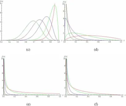
Here we have drawn some illustrative pdf of LLp(,) distributions for different choices
of parameters , and index p to study their shapes. It is observed that the distribution can be positively (negatively) skewed, symmetrical, and increasing (deceasing) type.
(c) (d)
(e) (f)
Figure 1. Pdf plots of LLp(,) when p = 0 (red), 1 (green), 3(blue), 5 (brown), 7
(light green) for (a) 20,0.001 (b) 5,0.1 (c) 20, 5 (d) 1
. 0 ,
2
(e) 0.5, 10 (f) 0.9,0 2.2Moment
Here we derive general result for moments of LLp(,) distribution and obtain its particular cases.
, 2, 1,1,2, ,
] 1
)[ 1 ( ) (
)) 2 ( ) 1 ( ) (( )
, ;
( 2
2
r
p p r
p p
r X
E p
p r
(13)
In particular,
p p X
E
p
1
) 1 ( 1 1
) , ; (
2
2.3 Mode
The mode plays an important role in the usefulness of a distribution. For the LLp(,)
distribution the mode occurs at
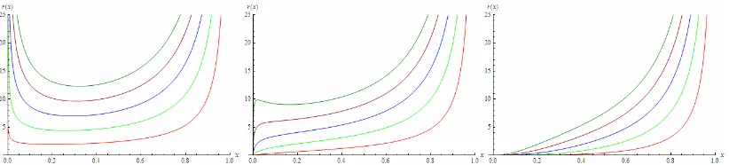
)] 2.4 Survival and Hazard Rate functions
] increasing and bath tub shaped.
log(log(1/ )
[log{( log ) }]LL which is the Log-Lindley (see proposition 2 in page 51 of Gomez et al., 2014). For integral values of index parameter p, exact expression for E
log(log(1/X)]
can be obtained using Mathematica as follows.
2.6 Stochastic Ordering
Theorem1. Let X1 and X2 be random variables following ( 1, 1)
1
p
LL and ( 2, 2)
2
p
LL
distributions, respectively. If 1 2,1 2 and p2 p1 then X1LR X2. Proof: Consider the ratio
) ( ) log ( ] 1
)[ 1 (
] 1
)[ 1 ( )
, , ; (
) , , ;
( 2 1
1 2
2 2 2 2
2 1
1 1 1 1
2 2 1 1 1
2 2 2
x h x p
p
p p
p x
f
p x
f p p
p p
(17)
where 2 1
log log )
(
1
2
x
x x x
h . Gomez-Deniz et al. (2014) has shown that the function )
(x
h is non-decreasing for x(0,1) if 12,12. Here, if p2 p1, it is clear that
1 2
) log
( x p p is non-decreasing for x(0,1). This implies that if 12,12 and
1
2 p
p , then the ratio in (17) is non-decreasing for x(0,1) and hence, X1LR X2. The result on LR ordering leads to the following (Gomez-Deniz et al., 2014):
2 1
2 1
2
1 X X X X X
X LR HR ST . Therefore, similar results as in Corollary 1 of Gomez-Deniz et al. (2014) can be shown for the new log-Lindley distribution as follows. Corollary 1. LetX1 and X2 be random variables following ( 1, 1)
1
p
LL and
) , ( 2 2
2
p
LL distributions, respectively. If 12,12 and p2 p1, then a. the moments, E[X1k]E[X2k] for all k 0;
b. the hazard rates, r1(x)r2(x) for all x(0,1).
2.7 Convexity and Concavity for Generalized Log-Lindley Distribution
For brevity, we suppress the cdf notation for LLp
, distribution in (5) as F(x) in this section.Theorem 2: If 0 1, p0 and 0, then F(x) is concave for x(0,1). Hence, for 0 1, F(x) is also log-concave for x(0,1) since F(x)0.
Proof: If 0 1, then (logx)p, (logx) and (x)1 are decreasing in x(0,1) for 0
,
3. Application to insurance premium loading
Proof: It has been shown in Theorem 2 that the cdf F(x;,) of LLp(,) is concave for 0 1.
Hence, 1F(1x;,) is a convex function from (0, 1) to (0, 1).
Remark: F(x;,) can be used as a distortion function to distort survival function (sf) of a given random variable as stated in the corollary below.
Corollary 2. If X is the risk with sf G(x) and let Z be a distorted random variable with survival function H(x)F[G(x);,] for 0 1andp0,0. Then
) ( ]
, ); ( [ ] [
0
x P dx x
G F Z
E
is a premium principle such that
i. P(X ) P,(X ) Pmax (X ) ii. P(axb)aP(x)b
iii. if X1 precedes X2under first stochastic dominance that is if G1(x1)G2(x2) then P,(X1)P,(X2)
iv. if X1 precedes X2 under second stochastic dominance that is if
2 0
2 2 1 0
1
1(x)dx G (x )dx
G
then P,(X1)P,(X2)
Where P(X)E(X)is the net premium/ average loss, Pmax(X) E[max{X1,,Xn}] is the maximum premium of the insurance product G1(x1)and G1(x1) are sf of two non negative risk r.v. respectively.
Proof: Since from theorem 2 above we know that F(x;,) is concave for x(0,1) when 0 1, p0 and 0 and is an increasing function of x with
0 ) , ; 0
(
F and F(1;,)1. Therefore by definition 6 of distortion premium principle and subsequent properties thereof in Wang (1996) the results follow immediately.
The log-likelihood function is then given by
For information matrix we obtain the following result The information matrix is given by
This matrix can be inverted to get asymptotic variance-covariance matrix for the maximum likelihood estimates.
5. Numerical Applications
In this section, for the purpose of application with the LLp
, regression model, re-parameterization of the distribution is required. The LLp
, will be re-parameterized in terms of its mean, in (14) together with two other new parameters and such that the parameters in (4) are replaced by:) parameterized log-Lindley distribution is obtained.
Suppose that a random sample Y1,Y2,,Yn of size n is obtained from the
,
LL distribution. For a set of k covariates, the logit link for the LL (,)
regression model gives the mean for each Y as
n i
T i T i
i , 1,2, ,
) exp( 1
) exp(
β β
x x
where xTi
1,xi1,,xik
are the covariates with corresponding coefficients
0,1,,k
β .
Here, the beta, LL and LL (,)regression models are applied on the data set originally used in Schmit and Roth (1990) and considered in Gomez-Deniz et al. (2014) about the cost effectiveness of risk management (measured in percentages) in relation to exposure to certain property and casualty losses, adjusted by several other variables such as size of assets and industry risk. Description on the data set may be found in Gomez-Deniz et al. (2014). We take the response variable to be y = FIRMCOST/100. Six other variables (covariates) are ASSUME (x1), CAP (x2), SIZELOG (x3), INDCOST (x4), CENTRAL (x5) and SOPH (x6). Similar to the analysis on the same data set by Jodra and Jimenez-Gamero (2016), who used a different re-parameterization of the Log-Lindley distribution, we investigated the cases of y and 1 – y with and without covariates.
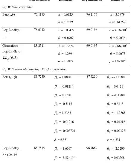
Table 1. Log-likelihood values and parameter estimates for beta, Log-Lindley and generalized Log-Lindley models, with and without covariates
Y 1 – y
Models
Log-likelihood Estimates Log-likelihood Estimates
(a) Without covariates
Beta(a,b) 76.1175 a = 0.6125
b = 3.7979
76.1175 a = 3.7979
b = 0.61252
Log-Lindley,
LL
76.6042 = 0.03427
= 0.6907
69.0196 = 4.16×103
= 5.9076
Generalized
Log-Lindley,
) , (
p LL
83.2511 = 0.3824
= 1.2694
p = 1.7819
69.0195 = 2.66×103
= 5.9077
p = 1.0×10⁻⁶
(b) With covariates and logit link for regression
Beta(,) 87.7230
0
= 1.8880
1
= -0.01214
2
= 0.1780
3
= -0.5115
4
= 1.2363
5
= -0.01216
6
= -0.003721
= 6.331
87.7230
0
= -1.8880
1
= 0.01214
2
= -0.1780
3
= 0.5115
4
= -1.2363
5
= 0.01216
6
= 0.003721
= 6.331
Log-Lindley,
) , (
1
LL
83.7575
0
= 1.6767
= -7.57×10⁻³
96.7689
0
= -2.7200
2
= 0.08903
3
= -0.4281
4
= 0.9687
5
= -0.02318
6
= 2.91×10-4
= 0.03488
2
= -0.7378
3
= 0.7024
4
= -3.7854
5
= 6.86×10⁻³
6
= 0.03593
= 67.212
Generalized
Log-Lindley,
) , (
LL
91.9525
0
= 0.2175
1
= 0.004907
2
= -0.1335
3
= -0.2644
4
= 0.4451
5
= -0.07726
6
= 0.005268
= 0.1755
γ = 2.6735
96.8252
0
= -2.7149
1
= 0.03221
2
= -0.7508
3
= 0.7049
4
= -3.7945
5
= 0.002473
6
= 0.03570
= 65.0001 γ = 1.0021
In terms of the log-likelihood values, it is clear from the results in Table 1 that the generalized Log-Lindley model fits the data best with or without covariates for the response variable y. It is also the best model for the regression of 1 – y, while the beta model is the best for this case without covariates. For the case of modeling 1 – y without covariates, it is seen that the estimates for the parameter p of the LLp
, modelapproaches 0 and hence, approaches the results for the LL distribution. Similarly for the regression of 1 – y with covariates, the estimates of the parameter γ for the LL
,6. Conclusion
A generalized Log-Lindley distribution has been investigated with important properties such as the pdf, cdf, survival function and hazard rate function derived. Application to a real life data set shows the relevance of the newly proposed distribution in regression modeling. The proposed distribution nests the Log Lindley distribution proposed by Gomez-Deniz et al. (2014).
References
1. G´omez−D´eniz, E, Sordo, M.A. and Calder´in−Ojeda, E (2014). The Log-Lindley distribution as an alternative to the beta regression model with applications in insurance, Insurance: Mathematics and Economics, 54, 49-57. 2. Jodra, P. and Jimenez-Gamero, M.D. (2016). A note on the Log-Lindley
distribution, Insurance: Mathematics and Economics, 71, 189-194.
3. Jones, M.C. (2009). Kumaraswamy’s distribution: a beta-type distribution with some tractability advantages, Statistical Methodology, 6, 70-81.
4. Nadaraja, S. (2005) Exponentiated Beta Distribution -, Computers and Mathematics with Application, 49, 1029-1035
5. Schmit, J.T., Roth, K. (1990). Cost effectiveness of risk managements practice. The Journal of Risk and Insurance 57 (3), 455–470.
6. Wang, S. (1996). Premium calculation by transforming the layer premium density, Astin Bulletin, 26 (1), 71-92.