Data Mashups
in R
by Jeremy Leipzig and Xiao-Yi Li Copyright © 2009 O’Reilly Media
ISBN: 9780596804770 Released: June 5, 2009
This article demonstrates how the real-world data is imported, managed, visual-ized, and analyzed within the R statisti-cal framework. Presented as a spatial mashup, this tutorial introduces the user to R packages, R syntax, and data struc-tures. The user will learn how the R en-vironment works with R packages as well as its own capabilities in statistical anal-ysis. We will be accessing spatial data in several formats—html, xml, shapefiles, and text—locally and over the web to produce a map of home foreclosure auc-tions and perform statistical analysis on these events.
Contents
Messy Address Parsing ... 2
Shaking the XML Tree ... 6
The Many Ways to Philly (Latitude) ... 8
Exceptional Circumstances ... 9
Taking Shape ... 11
Developing the Plot ... 14
Turning Up the Heat ... 17
Statistics of Foreclosure ... 19
Final Thoughts ... 28
Programmers can spend good part of their careers scripting code to conform to commercial statistics packages, visualization tools, and domain-specific third-par-ty software. The same tasks can force end users to spend countless hours in copy-paste purgatory, each minor change necessitating another grueling round of for-matting tabs and screenshots. R scripting provides some reprieve. Because this open source project garners support of a large community of package developers, the R statistical programming environment provides an amazing level of extensi-bility. Data from a multitude of sources can be imported into R and processed using R packages to aid statistical analysis and visualization. R scripts can also be configured to produce high-quality reports in an automated fashion - saving time, energy, and frustration.
This article will attempt to demonstrate how the real-world data is imported, managed, visualized, and analyzed within R. Spatial mashups provide an excellent way to explore the capabilities of R, giving glimpses of R packages, R syntax and data structures. To keep this tutorial in line with 2009 zeitgeist, we will be plotting and analyzing actual current home foreclosure auctions. Through this exercise, we hope to provide an general idea of how the R environment works with R packages as well as its own capabilities in statistical analysis. We will be accessing spatial data in several formats—html, xml, shapefiles, and text—locally and over the web to produce a map of home foreclosures and perform statistical analysis on these events.
Messy Address Parsing
To illustrate how to combine data from disparate sources for statistical analysis and visualization, let’s focus on one of the messiest sources of data around: web pages.
The Philadelphia Sheriff’s office posts foreclosure auctions on its website [http:// www.phillysheriff.com/properties.html] each month. How do we collect this data, massage it into a reasonable form, and work with it? First, let’s create a new folder (e.g. ~/Rmashup) to contain our project files. It is helpful to change the R working directory to your newly created folder.
#In Unix/MacOS
> setwd("~/Documents/Rmashup/")
#In Windows
> setwd("C:/~/Rmashup/")
We can download this foreclosure listings webpage from within R (you may choose instead to save the raw html from your web browser):
Here is some of this webpage’s source html, with addresses highlighted: <center><b> 258-302 </b></center>
84 E. Ashmead St.
    22nd Ward
974.96 sq. ft. BRT# 121081100 Improvements: Residential Property <br><b>
Homer Simpson    
</b> C.P. November Term, 2008 No. 01818     $55,132.65     Some Attorney & Partners, L.L.P.
<hr />
<center><b> 258-303 </b></center>
1916 W. York St.
    16th Ward
992 sq. ft. BRT# 162254300 Improvements: Residential Property
The Sheriff’s raw html listings are inconsistently formatted, but with the right reg-ular expression we can identify street addresses: notice how they appear alone on a line. Our goal is to submit viable addresses to the geocoder. Here are some typical addresses that our regular expression should match:
5031 N. 12th St.
2120-2128 E. Allegheny Ave. 1001-1013 Chestnut St., #207W 7409 Peregrine Place
3331 Morning Glory Rd. 135 W. Washington Lane
These are not addresses and should not be matched: 1,072 sq. ft. BRT# 344357100
</b> C.P. August Term, 2008 No. 002804
R has built-in functions that allow the use of perl-type regular expressions. (For more info on regular expressions, see Mastering Regular Expressions [http:// oreilly.com/catalog/9780596528126/], Regular Expression Pocket Refer-ence [http://oreilly.com/catalog/9780596514273]).
With some minor deletions to clean up address idiosyncrasies, we should be able to correctly identify street addresses from the mess of other data contained in properties.html. We’ll use a single regular expression pattern to do the cleanup. For clarity, we can break the pattern into the familiar elements of an address (number, name, suffix)
> stNum<-"^[0-9]{2,5}(\\-[0-9]+)?" > stName<-"([NSEW]\\. )?[0-9A-Z ]+"
Note the backslash characters themselves must be escaped with a backslash to avoid conflict with R syntax. Let’s test this pattern against our examples using
R’s grep() function:
> grep(myStPat,"3331 Morning Glory Rd.",perl=TRUE,value=FALSE,ignore.case=TRUE)
[1] 1
> grep(myStPat,"1,072 sq. ft. BRT#344325",perl=TRUE,value=FALSE,ignore.case=TRUE)
integer(0)
The result, [1] 1, shows that the first of our target address strings matched; we
tested only one string at a time. We also have to omit strings that we don’t want along with our address, such as extra quotes or commas, or Sheriff Office desig-nations that follow street names:
> badStrings<-"(\\r| a\\/?[kd]\\/?a.+$| - Premise.+$| assessed as.+$|, Unit.+|<font size=\"[0-9]\">|Apt\\..+| #.+$|[,\"]|\\s+$)"
Test this against some examples using R’s gsub() function:
> gsub(badStrings,'',"205 N. 4th St., Unit BG, a/k/a 205-11 N. 4th St., Unit BG", perl=TRUE)
[1] "205 N. 4th St."
> gsub(badStrings,'',"38 N. 40th St. - Premise A",perl=TRUE)
[1] "38 N. 40th St."
Let’s encapsulate this address parsing into a function that will accept an html file and return a vector [http://cran.r-project.org/doc/manuals/R-intro.html#Vec tors-and-assignment], a one-dimensional ordered collection with a specific data type, in this case character. Copy and paste this entire block into your R console:
#input:html filename
#returns:dataframe of geocoded addresses that can be plotted by PBSmapping getAddressesFromHTML<-function(myHTMLDoc){
myStPat<-paste(stNum,stName,stSuf,sep=" ") for(line in readLines(myHTMLDoc)){
line<-gsub(badStrings,'',line,perl=TRUE) matches<-grep(myStPat,line,perl=TRUE, value=FALSE,ignore.case=TRUE) if(length(matches)>0){
myStreets<-append(myStreets,line) }
myStreets }
We can test this function on our downloaded html file:
> streets<-getAddressesFromHTML("properties.html") > length(streets)
[1] 427
Exploring “streets”
R has very strong vector subscripting support. To access the first six foreclosures on our list:
> streets[1:6]
[1] "410 N. 61st St." "84 E. Ashmead St." "1916 W. York St." [4] "1216 N. 59th St." "1813 E. Ontario St." "248 N. Wanamaker St."
c() forms a vector from its arguments. Subscripting a vector with another vector
does what you’d expect: here’s how to form a vector from the first and last elements of the list.
> streets[c(1,length(streets))]
[1] "410 N. 61st St." "717-729 N. American St." Here’s how to select foreclosures that are on a “Place”:
> streets[grep("Place",streets)]
[1] "7518 Turnstone Place" "12034 Legion Place" "7850 Mercury Place" [4] "603 Christina Place"
Foreclosures ordered by street number, so dispense with non-numeric characters, cast as numeric, and use order() to get the indices.
> streets[order(as.numeric(gsub("[^0-9].+",'',streets)))] [427] "12854 Medford Rd."
Obtaining Latitude and Longitude Using Yahoo
http://local.yahooapis.com/MapsService/V1/geocode?ap pid=YD-9G7bey8_JXxQP6rxl.fBFGgCdNjoDMACQA--&street=1+South+Broad+St&city=Philadelphia&state=PA
In response we get: <?xml version="1.0"?>
<ResultSet xmlns:xsi="http://www.w3.org/2001/XMLSchema-instance" xmlns="urn:yahoo:maps"
xsi:schemaLocation=
"urn:yahoo:maps http://api.local.yahoo.com/MapsService/V1/GeocodeResponse.xsd"> <Result precision="address">
<Latitude>39.951405</Latitude> <Longitude>-75.163735</Longitude> <Address>1 S Broad St</Address> <City>Philadelphia</City> <State>PA</State>
<Zip>19107-3300</Zip> <Country>US</Country> </Result>
</ResultSet>
To use this service with your mashup, you must sign up with Yahoo! and receive an Application ID. Use that ID in with the ‘appid’ parameter of the request url. Sign up here: http://developer.yahoo.com/maps/rest/V1/geocode.html.
Shaking the XML Tree
Parsing well-formed and valid XML is much easier parsing than the Sheriff’s html. An XML parsing package is available for R; here’s how to install it from CRAN’s repository:
> install.packages("XML") > library("XML")
Warning
If you are behind a firewall or proxy and getting errors: On Unix: Set your http_proxy environment variable.
On Windows: try the custom install R wizard with internet2 option instead of “standard”. Click for additional info [http://cran.r-project.org/bin/
Our goal is to extract values contained within the <Latitude> and <Longitude> leaf
nodes. These nodes live within the <Result> node, which lives inside a <ResultSet> node, which itself lies inside the root node
To find an appropriate library for getting these values, call library(help=XML). This function lists the functions in the XML package.
> library(help=XML) #hit space to scroll, q to exit
> ?xmlTreeParse
I see the function xmlTreeParse will accept an XML file or url and return an R
structure. Paste in this block after inserting your Yahoo App ID. > library(XML)
> appid<-'<put your appid here>'
> street<-"1 South Broad Street"
> requestUrl<-paste(
"http://local.yahooapis.com/MapsService/V1/geocode?appid=", appid,
"&street=",
URLencode(street),
"&city=Philadelphia&state=PA" ,sep="")
> xmlResult<-xmlTreeParse(requestUrl,isURL=TRUE)
Warning
Are you behind a firewall or proxy in windows and this example is giving you trouble?
xmlTreeParse has no respect for your proxy settings. Do the following:
> Sys.setenv("http_proxy" = "http://myProxyServer:myProxyPort")
or if you use a username/password
> Sys.setenv("http_proxy"="http://username:password@proxyHost:proxyPort″)
You need to install the cURL package to handle fetching web pages
> install.packages("RCurl") > library("RCurl")
in the example above change:
> xmlResult<-xmlTreeParse(requestUrl,isURL=TRUE)
to:
> xmlResult<-xmlTreeParse(getURL(requestUrl))
the jugular by using what we can gleam from the data structure that
.. .. .. .. ..- attr(*, "class")= chr [1:5] "XMLTextNode" "XMLNode" "RXMLAb... .. .. .. ..- attr(*, "class")= chr [1:4] "XMLNode" "RXMLAbstractNode" "XMLA... .. .. ..$ Longitude:List of 1
.. .. .. ..$ text: list()
.. .. .. .. ..- attr(*, "class")= chr [1:5] "XMLTextNode" "XMLNode" "RXMLAb... .. .. .. ..- attr(*, "class")= chr [1:4] "XMLNode" "RXMLAbstractNode" "XMLA...
(snip)
That’s kind of a mess, but we can see our Longitude and Latitude are Lists inside of Lists inside of a List inside of a List.
Tom Short’s R reference card, an invaluable handy resource, tells us to get the element named name in list X of a list in R x[['name']]: http://cran.r-project.org/ doc/contrib/Short-refcard.pdf.
The Many Ways to Philly (Latitude)
Using Data Structures
Using the indexing list notation from R we can get to the nodes we need
> lat<-xmlResult[['doc']][['ResultSet']][['Result']][['Latitude']][['text']] > long<-xmlResult[['doc']][['ResultSet']][['Result']][['Longitude']][['text']]
> lat
39.951405
looks good, but if we examine this further
> str(lat)
list()
- attr(*, "class")= chr [1:5] "XMLTextNode" "XMLNode" "RXMLAbstractNode" "XML...
Although it has a decent display value this variable still considers itself an XMLNode and contains no index to obtain raw leaf value we want—the descriptor just says list() instead of something we can use (like $lat). We’re not quite there
yet.
Using Helper Methods
> lat<-xmlValue(xmlResult[['doc']][['ResultSet']][['Result']][['Latitude']])
> str(lat)
chr "39.951405"
Using Internal Class Methods
There are usually multiple ways to accomplish the same task in R. Another means to get to this our character lat/long data is to use the “value” method provided by the node itself
> lat<-xmlResult[['doc']][['ResultSet']][['Result']][['Latitude']][['text']]$value
If we were really clever we would have understood that XML doc class provided us with useful methods all the way down! Try neurotically holding down the tab key after typing
> lat<-xmlResult$ (now hold down the tab key)
xmlResult$doc xmlResult$dtd
(let's go with doc and start looking for more methods using $)
> lat<-xmlResult$doc$
After enough experimentation we can get all the way to the result we were looking for
> lat<-xmlResult$doc$children$ResultSet$children
$Result$children$Latitude$children$text$value
> str(lat)
chr "39.951405"
We get the same usable result using raw data structures with helper methods, or internal object methods. In a more complex or longer tree structure we might have also used event-based or XPath-style parsing to get to our value. You should always begin by trying approaches you find most intuitive.
Exceptional Circumstances
The Unmappable Fake Street
Now we have to deal with the problem of bad street addresses—either the Sheriff office enters a typo or our parser lets a bad street address pass: http://local.ya hooapis.com/MapsService/V1/geocode?ap
pid=YD-9G7bey8_JXxQP6rxl.fBFGgCdNjoDMACQA--&street=1+Fake +St&city=Philadelphia&state=PA.
Note the “precision” attribute of the result is “zip” instead of address and there is
warning="The street could not be found. Here is the center of the city."> <Latitude>39.952270</Latitude>
> street<-"1 Fake St" > requestUrl<-paste(
"http://local.yahooapis.com/MapsService/V1/geocode?appid=", appid,
"&street=",
URLencode(street),
"&city=Philadelphia&state=PA" ,sep="")
We need to get a hold of the attribute tags within <Result> to distinguish bad geocoding events, or else we could accidentally record events in the center of the city as foreclosures. By reading the RSXML FAQ [http://www.omegahat.org/ RSXML/FAQ.html] it becomes clear we need to turn on the addAttributeNames-paces parameter to our xmlTreeParse call if we are to ever see the precision tag.
> xmlResult<-xmlTreeParse(requestUrl,isURL=TRUE,addAttributeNamespaces=TRUE)
Now we can dig down to get that precision tag, which is an element of $attributes, a named list
> xmlResult$doc$children$ResultSet$children$Result$attributes['precision']
precision "zip"
We can add this condition to our geocoding function:
}else{
cat("I don't know where this is!\n") }
No Connection
Finally we need to account for unforeseen exceptions—such as losing our internet connection or the Yahoo web service failing to respond. It is not uncommon for this free service to drop out when bombarded by requests. A try-catch clause will alert us if this does happen and prevent bad data from getting into our results.
> tryCatch({
xmlResult<-xmlTreeParse(requestUrl,isURL=TRUE,addAttributeNamespaces=TRUE)
#...other code...
}, error=function(err){
cat("xml parsing or http error:", conditionMessage(err), "\n") })
We will compile all this code into a single function once we know how to merge it with a map (see Developing the Plot).
Taking Shape
Finding a Usable Map
To display a map of Philadelphia with our foreclosures, we need to find a polygon of the county as well as a means of plotting our lat/long coordinates onto it. Both these requirements are met by the ubiquitous ESRI shapefile format. The term shapefile [http://en.wikipedia.org/wiki/Shapefile] collectively refers to a .shp file, which contains polygons, and related files which store other features, indices, and metadata.
Googling “philadelphia shapefile” returns several promising results including this page: http://www.temple.edu/ssdl/Shape_files.htm.
PBSmapping
PBSmapping is a popular R package that offers several means of interacting with spatial data. It relies on some base functions from the maptools package to read ESRI shapefiles, so we need both packages.
> install.packages(c("maptools","PBSmapping"))
As with other packages we can see the functions using
library(help=PBSmapping) and view function descriptions using ?topic: http://
cran.r-project.org/web/packages/PBSmapping/index.html.
We can use str to examine the structure of the shapefile imported by
PBSmapping::importShapeFile > library(PBSmapping)
PBS Mapping 2.59 Copyright (C) 2003-2008 Fisheries and Oceans Canada PBS Mapping comes with ABSOLUTELY NO WARRANTY; for details see the
file COPYING. This is free software, and you are welcome to redistribute it under certain conditions, as outlined in the above file.
A complete user's guide 'PBSmapping-UG.pdf' appears in the '.../library/PBSmapping/doc' folder.
To see demos, type '.PBSfigs()'. Built on Oct 7, 2008
Pacific Biological Station, Nanaimo
> myShapeFile<-importShapefile("tracts2000",readDBF=TRUE)
Loading required package: maptools Loading required package: foreign Loading required package: sp
> str(myShapeFile)
- attr(*, "PolyData")=Classes 'PolyData' and 'data.frame': 381 obs. of 9 var... ..$ PID : int 1 2 3 4 5 6 7 8 9 10 ...
..$ ID : Factor w/ 381 levels "1","10","100",..: 1 112 223 316 327 338... ..$ FIPSSTCO: Factor w/ 1 level "42101": 1 1 1 1 1 1 1 1 1 1 ...
..$ TRT2000 : Factor w/ 381 levels "000100","000200",..: 1 2 3 4 5 6 7 8 9 ... ..$ STFID : Factor w/ 381 levels "42101000100",..: 1 2 3 4 5 6 7 8 9 10 ... ..$ TRACTID : Factor w/ 381 levels "1","10","100",..: 1 114 226 313 327 337... ..$ PARK : num 0 0 0 0 0 0 0 0 0 0 ...
..$ OLDID : num 1 1 1 1 1 1 1 1 1 1 ... ..$ NEWID : num 2 2 2 2 2 2 2 2 2 2 ...
- attr(*, "shpType")= int 5 - attr(*, "prj")= chr "Unknown" - attr(*, "projection")= num 1
While the shapefile itself consists of 16290 points that make up Philadelphia, it appears a lot of the polygon data associated with this shapefile is stored in as an attribute of myShapeFile. We should set that to a top level variable for easier access. > myPolyData<-attr(myShapeFile,"PolyData")
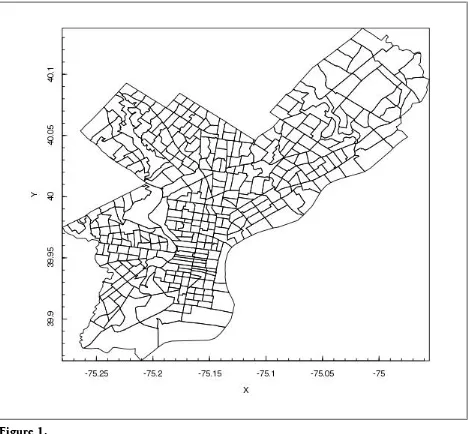
Plotting this valid shapefile is remarkably easy (see Figure 1):
> plotPolys(myShapeFile)
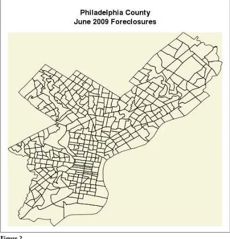
Let’s spruce that up a bit (see Figure 2):
> plotPolys(myShapeFile,axes=FALSE,bg="beige",main="Philadelphia County\n June 2009 Foreclosures",xlab="",ylab="")
Developing the Plot
Preparing to Add Points to Our Map
To use the PBSmapping’s addPoints function, the reference manual suggests we
treat our foreclosures as "EventData“. The EventData format is a standard R data
frame (more on data frames below) with required columns X, Y, and a unique row identifier EID. With this in mind we can write a function around our geocoding code that will accept a list of streets and return a kosher EventData-like dataframe.
#input:vector of streets
#output:data frame containing lat/longs in PBSmapping-like format
> geocodeAddresses<-function(myStreets){ 'appid<-'<put your appid here>' myGeoTable<-data.frame(
address=character(),lat=numeric(),long=numeric(),EID=numeric()) for(myStreet in myStreets){
requestUrl<-paste(
"http://local.yahooapis.com/MapsService/V1/geocode?appid=", appid,
"&street=",URLencode(myStreet), "&city=Philadelphia&state=PA",sep="") cat("geocoding:",myStreet,"\n") tryCatch({
xmlTreeParse(requestUrl,isURL=TRUE,addAttributeNamespaces=TRUE) geoResult<-xmlResult$doc$children$ResultSet$children$Result if(geoResult$attributes['precision'] == 'address'){
lat<-xmlValue(geoResult[['Latitude']])
cat("xml parsing/http error:", conditionMessage(err), "\n") })
Sys.sleep(0.5) #this pause helps keep Yahoo happy }
#use built-in numbering as the event id for PBSmapping myGeoTable$EID<-as.numeric(rownames(myGeoTable))
myGeoTable }
After pasting the above geocodeAddresses function into your R console, enter in
the following (make sure you still have a streets vector from the parsing chapter):
> geoTable<-geocodeAddresses(streets) geocoding: 410 N. 61st St.
geocoding: 84 E. Ashmead St. geocoding: 1916 W. York St. geocoding: 1216 N. 59th St. geocoding: 1813 E. Ontario St. geocoding: 248 N. Wanamaker St. geocoding: 3469 Eden St.
geocoding: 2039 E. Huntingdon St.
...(snip)...
geocoding: 4935 Hoopes St.
Exploring R Data Structures: geoTable
> names(geoTable)
X and Y from the first five rows:
> geoTable[1:5,c("X","Y")]
Cell at 4th column, 4th row
> geoTable[4,4]
[1] 4
Second column, also known as “Y”
> geoTable[,2]
#or#
> geoTable$Y
[1] 39.96865 40.03168 39.99043 39.97047 39.99882 39.96542 40.06410 39.98569 [9] 39.99738 39.93542 40.04451 39.92172 39.96829 39.94470 40.01606 39.96614
...
With lat/longs in hand it is easy for R to describe our foreclosure data. What is the northernmost (highest latitude) of our foreclosures?
> geoTable[geoTable$Y==max(geoTable$Y),]
address Y X EID 315 12338 Wyndom Rd. 40.10177 -74.97684 315
Making Events of our Foreclosures
Our geoTable is similar in structure to an EventData object but we need to use to
the as.EventData function to complete the conversion.
> addressEvents<-as.EventData(geoTable,projection=NA)
Error in as.EventData(geoTable, projection = NA) : Cannot coerce into EventData.
Oh snap! The dreaded “factor feature” in R strikes again. When a data frame col-umn contains factors [ http://cran.r-project.org/doc/manuals/R-lang.html#Factors], its elements are represented using indices that refer to levels, distinct values within that column. The as.EventData method is expecting columns
of type numeric, not factor.
Never transform from factors to numeric like this:
as.numeric(myTable$factorColumn) #don't do this!
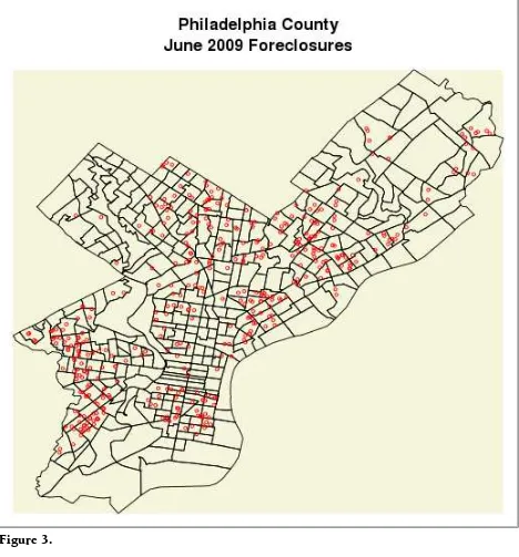
An extremely common mistake—this will merely return numeric indicies used to refer to the levels—you want the levels themselves (Figure 3).
> geoTable$X<-as.numeric(levels(geoTable$X))[geoTable$X] #do this
> geoTable$Y<-as.numeric(levels(geoTable$Y))[geoTable$Y]
> addressEvents<-as.EventData(geoTable,projection=NA) > addPoints(addressEvents,col="red",cex=.5)
Turning Up the Heat
PBSmapping allows us to see which in polygons/tracts our foreclosures were plot-ted. Using this data we can represent the intensity of foreclosure events as a heat-map.
Each EID (event id aka foreclosure) is associated with a PID (polygon id aka tract). To plot our heatmap we need to count instances of PIDs in addressPolys for each
tract on the map.
> length(levels(as.factor(myShapeFile$PID)))
> length(levels(as.factor(addressPolys$PID)))
[1] 196
We can see there are 381 census tracts in Philadelphia but only 196 have foreclosure events. For the purpose of coloring our polygons we need to insure remainder are explicitly set to 0 foreclosures.
The table function in R can be used to make this sort of contingency table. We need a variable, myTrtFC, to hold the number forclosures in each tract/PID:
>
table(factor(addressPolys$PID,levels=levels(as.factor(myShapeFile$PID))))
> myTrtFC
1 2 3 4 5 6 7 8 9 10 11 12 13 14 15 16 17 18 19 20 1 0 1 1 0 0 0 0 0 0 0 0 2 3 0 0 3 1 1 1
(snip)
(To enforce our new levels we must use a constructor (factor) instead of a variable
conversion (as.factor))
Filling with Color Gradients
R has some decent built-in color gradient functions (?rainbow to learn more)—we
will need a different color for each non-zero level plus one extra for zero foreclo-sures.
> mapColors<-heat.colors(max(myTrtFC)+1,alpha=.6)[max(myTrtFC)-myTrtFC+1]
Our plot is virtually the same but we add the color vector argument (col). We can
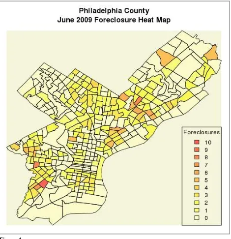
easily add a legend with the sequence 10 through 0 foreclosures and its corre-sponding heat levels (Figure 4).
> plotPolys(myShapeFile,axes=FALSE,bg="beige",main="Philadelphia County\n June 2009 Foreclosure Heat Map",xlab="",ylab="",col=mapColors) > legend("bottomright",legend=max(myTrtFC):0,
fill=heat.colors(max(myTrtFC)+1,alpha=.6), title="Foreclosures")
Statistics of Foreclosure
The same parsing, rendering of shapefiles, and geocoding of foreclosure events reviewed up to this point can be done in a number of other platforms. The real strength of R is found in its extensive statistical functions and libraries.
Importing Census Data
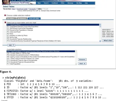
The US Census Bureau collects an extensive range of socioeconomic data that are interesting for our purposes. We can download some data involved in total pop-ulation and total housing units that are indexed by the same tracts we have used for our map. FactFinder download center [http://factfinder.census.gov/serv let/DCGeoSelectServlet?ds_name=DEC_2000_SF3_U ] provides easy access to these data, as shown in Figure 5.
Then, select All Census Tracts in a County→Pennsylvania→Philadelphia Coun-ty→Selected Detailed Tables, as shown in Figure 6.
Add the eight tables (P1,P13, P14, P31, P41, P53, P87,H33), click next, download, and unzip the file.
> censusTable1<-read.table("dc_dec_2000_sf3_u_geo.txt",sep="|",header=TRUE) > censusTable2<-read.table("dc_dec_2000_sf3_u_data1.txt",sep="|", header=TRUE, skip=1, na.string="")
> colnames(censusTable2)
[1] "Geography.Identifier" [2] "Geography.Identifier.1" [3] "Geographic.Summary.Level" [4] "Geography"
[5] "Total.population..Total" [6] "Households..Total"
[7] "Households..Family.households"
[8] "Households..Family.households..Householder.15.to.24.years"
[9] "Households..Family.households..Householder.25.to.34.years" [10] "Households..Family.households..Householder.35.to.44.years" [11] "Households..Family.households..Householder.45.to.54.years" [12] "Households..Family.households..Householder.55.to.64.years" [13] "Households..Family.households..Householder.65.to.74.years" [14] "Households..Family.households..Householder.75.to.84.years" [15] "Households..Family.households..Householder.85.years"...
Examining our downloaded data, we see that the first line in the text file are IDs that makes little sense, while the second line describes the IDs. The skip=1 option
in read.table allow us to skip the first column, By skipping the first line, the headers of censusTable are extracted from the second line. Also notice, one of R’s quirks is that it likes to replace spaces with a period.
The columns we need are in different tables. CensusTable1 contains the tracts, CensusTable2 has all the interesting survey variables, while FCs and polyData have
foreclosure and shape information. The str() and merge() function can be quite
useful in this case. The Geography.Identifier.1 in the censusTable2 looks familiar
—it matches with STFID from the PolyData table extracted from our shapefile.
> str(myPolyData)
Classes 'PolyData' and 'data.frame': 381 obs. of 9 variables: $ PID : int 1 2 3 4 5 6 7 8 9 10 ...
$ ID : Factor w/ 381 levels "1","10","100",..: 1 112 223 316 327 ... $ FIPSSTCO: Factor w/ 1 level "42101": 1 1 1 1 1 1 1 1 1 1 ...
$ TRT2000 : Factor w/ 381 levels "000100","000200",..: 1 2 3 4 5 6 7 ... $ STFID : Factor w/ 381 levels "42101000100",..: 1 2 3 4 5 6 7 8 9 10 ...
(snip)
#selecting columns with interesting data
> ct1<-censusTable2[,c(1,2,5,6,7,16,42,54,56,75,76,77,93,94,105)]
#merge function can merge two tables at a time
> ct2<-merge(x=censusTable1,y=myPolyData, by.x='GEO_ID2', by.y='STFID') > ct3<-merge(x=ct2, y=ct1, by.x='GEO_ID2', by.y='Geography.Identifier.1')
Now we have a connection between the tracts and our census data. We need to also include the foreclosure data. We have myTrtFC, but it would be easier to do
another merge if it was a data frame.
> myTrtFC<-as.data.frame(myTrtFC) > names(myTrtFC)<-c("PID","FCs")
> ct<-merge(x=ct3,y=myTrtFC,by.x="PID",by.y="PID")
Changing the names for each column will facilitate scripting later on. Of course, it’s just a personal preference.
> colnames(ct)<-c("PID", "GEO_ID", "GEO_ID2", "SUMLEV", "GEONAME", "GEOCOMP", "STATE", "COUNTY", "TRACT", "STATEP00", "COUNTYP00", "TRACTCE00", "NAME00", "NAMELSAD00", "MTFCC00", "FUNCSTAT00", "Geography.Identifier", "totalPop", "totalHousehold", "familyHousehold", "nonfamilyHousehold", "TravelTime", "TravelTime90+minutes", "totalDisabled", "medianHouseholdIncome",
"povertyStatus", "BelowPoverty","OccupiedHousing", "ownedOccupied", "rentOccupied", "FCS")
Descriptive Statistics
Calculating mean, median, and standard deviation in R are quite intuitive. They are simply mean(), median(), and sd(). To perform multiple means, medians, etc
at the same time use summary() > summary(ct)
#na.rm=TRUE is necessary if there are missing data #in the standard deviation calculations.
#The size will be only available data.
PID Geography.Identifier.1
Not all of the columns will return a numeric value, especially if it’s missing. For example, MTFCC00 returns a NA. Its type is considered as a factor, as opposed
to a num or int (see output from str() from above). The na.rm=TRUE in the sd
func-tion removes missing data. It also follows a warning : Warning messages:
1: In var(as.vector(x), na.rm = na.rm) : NAs introduced by coercion
The warning serves to alert the user that that column is not of num or int type. Of
course, the standard deviations of MTFCC00 or FUNCSTAT00 are nonsensical and hence uninteresting to calculate. In this case, we can ignore the warning mes-sage.
> cor(ct[,c(18,19)], method="pearson", use="complete")
totPop totHousehold totPop 1.0000000 0.9385048 totHousehold 0.9385048 1.0000000
cor has a default method using Pearson’s test statistic, calculating the shortest
“distance” between each of the pairwise variables. Total population and household families are very close to each other, thus have a R-squared value of 0.94. The ‘use="complete"' option suggests that only those variables with no missing values should be used to find correlation. The other option is pairwise.
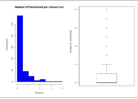
table() is a good way to look at the frequency distribution.
> table(ct$FCS)
0 1 2 3 4 5 6 7 8 203 84 46 25 6 11 2 2 2
Two of the 381 tracts have 8 foreclosures. And 203 tracts have no foreclosures. Another more visually pleasing way to look at the foreclosure data would be his-tograms
Descriptive Plots
Let’s create a new subset of the table that only includes covariates and foreclosure. Can we find any associations between the attributes of each tract and its foreclo-sures? $ medianHouseholdIncome: int 48886 8349 40625 27400 9620 41563 34536 42346 ... $ BelowPoverty : int 223 690 236 666 332 176 454 1218 1435 370 ... $ OccupiedHousing : int 2378 1171 1941 3923 372 786 2550 8446 4308 ... $ FCS : int 1 0 1 1 0 0 0 0 0 0 ...
Histograms are the graphical representation of the same results we obtained from
table(). The boxplots are the graphical representation of the results obtatined
from summary() (if the variable is numeric). Both are visual representations of the
distribution of the variable in question. Let’s use the foreclosure (FCS) variable:
> attach(corTable1) #lets R know that the variable below will be from
> par(mfrow=c(2,1)) # makes it easy to view multiple graphs in one window
> boxplot(FCS, ylab="Number of Foreclosures") > detach(corTable1) # the table is no longer attached
The results from these graphs are show in Figure 7.
Correlation Revisited
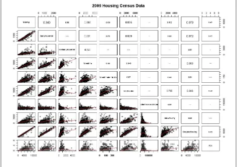
Correlation is a basic statistic used frequently by researchers and statisticians. In R, we can create multidimensional correlation graphs using the pairs() scatterplot
matrix package. The following code will enhance pairs() by allowing the upper
triangle to show the actual correlation numbers, while the lower triangle to show correlation plots:
#first create a function (panel.cor) for the upper triangle
> panel.cor <- function(x, y, digits=3, prefix="", cex.cor){ usr <- par("usr"); on.exit(par(usr))
par(usr = c(0, 1, 0, 1))
r = (cor(x, y, method="pearson", use="complete")) txt <- format(c(r, 0.123456789), digits=digits)[1] txt <- paste(prefix, txt, sep="")
if(missing(cex.cor)) cex <- 0.8/strwidth(txt) text(0.5, 0.5, txt, cex = cex * abs(r)) }
#now plot using pairs()
> pairs(corTable1, lower.panel=panel.smooth,
upper.panel=panel.cor, main="2009 Housing Census Data",
labels=c("TotPop","Families","HouseholdIncome","House Units", "Occupied House", "Vacant House", "OwnerOccupied House Mortgage",
"OwnerOccupied House W/O Mortgage"), font.labels=2)
The resulting graph is shown in Figure 8.
From the above plot, we observe total population, total families households and total housing units are all highly correlated as would be expected. We also observe that median household income, total travel time, number of occupants below poverty level and number of non-family households are not correlated with each other or any of the other variables.
One interesting observation is the correlation between the total population and the median household income.
There are one or two less populated tracts whose household income is also quite high, while the remainder follow a linear trend. The median household income
appears constant across all tracts regardless of the total population in each tract. For other variables, the tracts with a high number of individuals below the poverty level tend to have median household incomes at the lower end of the range. Such a clumping trend is also observed between those with low income. There is a non-linear relationship between foreclosure rates and median income, where tracts above a certain income threshold experience almost no foreclosure events.
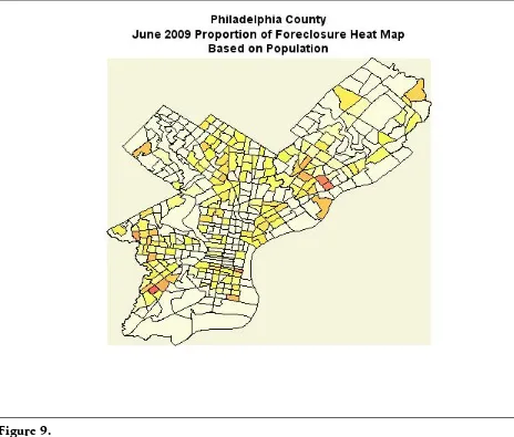
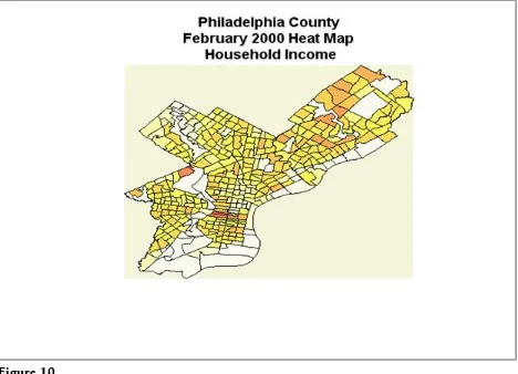
Each data point is the frequency of a particular geographical location. This data can be used to create the heatmaps shown Figure 9 in using the same steps men-tioned above.
The heatmaps above do show very few foreclosures for those tracts with high household incomes. Further statistical analysis might include association of fore-closure and household income. Such specific regression analysis will not be cov-ered in this article.
Final Thoughts
R users rely on packages to do complex tasks without heavy scripting. Using these packages effectively usually requires some trial-and-error, but R package usage patterns will typically resemble what has been covered in this tutorial. In addition to reviewing the internal help and examples, it is good practice to closely examine each package’s data structures using str(). The interactive nature of R allows a
beginner to attempt to solve complex problems by trying different strategies in real-time without the hassles of compilation. A spatial mashup cannot cover R’s extensive statistical capabilities, but hopefully this tutorial will spark some interest in programmers who want to incorporate statistical analysis into their data pipe-lines.
Appendix: Getting Started
Obtaining R
R is available here: http://cran.r-project.org/.
Consoles with a limited but handy menu come with the Windows and Mac dis-tributions. These make browsing available packages and documentation some-what easier. In Unix, the R executable will generally install into /usr/bin/R and uses x11 windows for graphs.
The commands in this tutorial work for all R platforms.
Quick and Dirty Essentials of R
Upon starting R, you will see a prompt describing the version of R you are access-ing, a disclaimer about R as a free software, and some functions regarding license, contributors and demos of R.
R uses an interactive shell—each line is interpreted after you hit return. A '>' prompt appears when R is ready for another command. In this tutorial, all com-mands that a user enters appear in bold after the prompt.
Built-in functions and simple mathematical calculations are the basics of R lan-guage. By typing 1+1 and hitting enter, you’ll observe the following:
> 1+1
[1] 2
> myAnswer<-sqrt(81) > myAnswer
[1] 9
Just like a calculator, you can also take logs log(), find the sin of angles sin(), and
take absolute values of any real number abs(). R allows you to store your results
in a variable by using the " <-" operator. To view the value of a variable, simply
type its name. Names in R are case-sensitive, so one, One, and oNe are three dif-ferent variables. You can also create a vector (a collection of elements) using var-iables of the same type (int, num, etc):
> x<-c(0,1,2,3) # R treats everything behind the pound sign as comments x [1] 0 1 2 3
> x[1] #access to the first element of the vector [1] 0
To view the internal help page for a unfamiliar function, type the keyword with ?. It will provide a detailed description of the function, its parameters, its
outputs and generally followed by a simple example using the function. You can also type help.search() to determine if there is a function that will perform what
you desire.
> ?mean
![Figure 5. [9] "Households..Family.households..Householder.25.to.34.years"](https://thumb-ap.123doks.com/thumbv2/123dok/1307277.2010045/21.612.72.541.67.425/figure-households-family-households-householder-years.webp)