Summary Mountain ash (Eucalyptus regnans F.J. Muell.) forest catchments exhibit a strong relationship between stand age and runoff, attributed inter alia to differences in tree water use. However, the tree water use component of the mountain ash forest water balance is poorly quantified. We have used the sap flow technique to obtain estimates of daily water use in large mountain ash trees. First, the sap flow technique was validated by means of an in situ cut tree experiment. Close agreement was obtained between the sap flow estimate of water use and the actual uptake of water by the tree from a reservoir. Second, we compared the variability in sap velocity between a symmetric and an asymmetric tree by using multiple sap flow loggers. In the symmetric tree, velocity was fairly uniform throughout the xylem during the day, indicating that accurate sap flow estimates can be obtained with a minimal number of sampling points. However, large variations in sap velocity were observed in the asymmetric tree, indicating that much larger sampling sizes are required in asymmetric stems for an accurate determination of mean sap velocity. Finally, we compared two procedures for scaling individual tree sap flow estimates to the stand level based on stem diameter and leaf area index meas-urements. The first procedure was based on a regression be-tween stem diameter and tree water use, developed on a small sample of trees and applied to a stand-level census of stem diameter values. Inputs to the second procedure were tree water use and leaf area of a single tree and the leaf area index of the stand. The two procedures yielded similar results; however, the first procedure was more robust but it required more sampling effort than the second procedure.
Keywords: Eucalyptus regnans, flow variability, forest catch-ment, runoff, sap velocity, stand age.
Introduction
The city of Melbourne’s water is harvested from 1550 km2 of forested catchments in the Central Highlands of Victoria, Aus-tralia. Mountain ash (Eucalyptus regnans F.J. Muell.) trees cover about half this area, but the area that they occupy yields 80% of the stream flow because it receives higher rainfall. It
has been established that re-growth mountain ash forests yield significantly less water than old-growth stands, partly because of differences in forest density and structure (Langford 1976, Kuczera 1987, Jayasuriya et al. 1993, Vertessy et al. 1994). However, the tree water use component of the mountain ash forest water balance remains poorly quantified. The main rea-son for this is that the mountain ash forests are very tall (up to 90 m) and grow in steep and variable terrain, thereby making micrometeorological techniques difficult to apply. The recent development of the sap flow measurement technique has helped overcome this problem (cf. Dunn and Connor 1993, Vertessy et al. 1995).
To date, two major sap flow measurement experiments have been carried out in mountain ash forest. Dunn and Connor (1993) found that the mean daily sap velocity of multiple trees within mountain ash stands of different ages did not vary significantly with respect to age when averaged over a 5--6-month period. They estimated mean daily sap velocities of 0.032, 0.032, 0.027 and 0.033 mm s−1 for 50-, 90-, 150- and 230-year-old mountain ash stands, respectively, over spring--summer, and attributed differences in water use amongst the different aged stands to differences in sapwood area. The sapwood values for the four age classes were 6.74, 6.09, 4.23 and 4.04 m2 ha−1, respectively. Vertessy et al. (1995) demon-strated that mean daily sap flow in nineteen 15-year-old moun-tain ash trees was closely related to the stem diameters and canopy leaf areas of the trees. They argued that similar rela-tionships should be derived for older stands to help elucidate the factors underlying the stand age--water yield relationship in mountain ash forests. Vertessy et al. (1995) also found that mean daily sap velocity (measured over a month in spring) varied considerably amongst trees in the stand, whereas the stand mean was 0.033 mm s−1. This finding supports the contention of Dunn and Connor (1993) that stand mean sap velocity does not vary significantly between mountain ash forests of different ages when measured over a suitably long period.
Although these two studies have shown that the sap flow measurement method can be used to quantify the mountain ash forest water balance more accurately than before, there are
Estimating stand water use of large mountain ash trees and validation
of the sap flow measurement technique
R. A. VERTESSY,
1,4T. J. HATTON,
1P. REECE,
1,4S. K. O’SULLIVAN
2,4and R. G. BENYON
3,41
CSIRO Land and Water, GPO Box 1666, Canberra, ACT 2601, Australia 2 Monash University, Wellington Road, Clayton, Victoria 3168, Australia
3
Melbourne Water, Box 4342, Melbourne, Victoria 3001, Australia 4
Cooperative Research Center for Catchment Hydrology, GPO Box 1666, Canberra, ACT 2601, Australia
Received November 13, 1996
several aspects of the technique that require further evaluation. The specific objectives of this study were: (1) to provide a comprehensive validation of the sap flow measurement method in mountain ash trees; (2) to determine sap velocity variability in mountain ash trees for use in the development of an optimal strategy for estimating mountain ash stand water use with the sap flow method in these forests; (3) to evaluate the relationships between sap flow and scalar variables such as stem diameter and leaf area for older stands of mountain ash; and (4) to optimize the method for scaling sap flow estimates for individual trees to an areal basis. Vertessy et al. (1995) used stem diameter measurements to scale up individual tree water use to the stand level, but it is unclear whether this is the optimum scaling method for mountain ash forests. We also discuss the contribution of our findings to the elucidation of the mountain ash forest age--water use relationship.
Materials and methods
Site description
All field measurements were made in an even-aged 56-year-old mountain ash stand that had regenerated naturally from seed after a wildfire destroyed the old-growth mountain ash forest in 1939. The stand is located at Black Spur in the North Maroondah Experimental Area, now part of the Yarra Ranges National Park, approximately 100 km NE of the city of Mel-bourne, Australia (145°38′ E, 37°34′ S), at an elevation of 750 m. Mean annual rainfall is 1660 mm, evenly distributed throughout the year with a slight spring maximum. Mean monthly temperatures vary between 3--5 °C in winter and 16--17 °C in summer. Mean monthly solar radiation for the site varies between 120 MJ m−2 in winter and 630 MJ m−2 in summer. Soils in the area are deep krasnozems of high perme-ability (up to 10 m day−1) and high water-holding capacity (soil water storage exceeding 5000 mm) (Langford and O’Shaughnessy 1977, Davis et al. 1996).
Sap flow nomenclature
We have adopted the unified nomenclature for sap flow meas-urements proposed by Edwards et al. (1997). The term sap velocity is used to denote the speed of water movement through the stem, expressed on a total sapwood area basis. The term sap flow denotes the volume of water moving through the stem per unit time (i.e., the product of sap velocity and sapwood area). Sap velocity (vs) is expressed in units of mm s−1 and sap flow (Q) is expressed in units of m3 day−1.
Cut tree experiment
We tested the sap flow measurement method by means of a cut tree experiment (sensu Landsberg et al. 1976, Roberts 1977, Olbrich 1991), performed on a radially uniform tree of 69 cm dbh (diameter at breast height over bark) and 65 m height. The average sapwood thickness of the tree was 32 mm, resulting in a total sapwood area of 396 cm2. The crown leaf area, deter-mined by destructive sampling after the experiment, was 163 m2.
A triangular wooden stand was constructed around the tree to support a water reservoir at 1.5 m above ground level. The reservoir was fabricated from a Class-A evaporation pan; we cut an 80-cm diameter hole in its center and fitted the inner hole with a rubber membrane (Figure 1). The pan was cut into two halves; these were placed on the stand around the stem of the tree, riveted back together and sealed. The rubber mem-brane was then strapped to the trunk of the tree and coated with silicon sealant. The whole internal surface of the pan and the tree trunk (up to the water line) were then covered with a thick coat of bituminous waterproof paint. When fitted around the tree, the reservoir had a storage capacity of 210 l.
Once the bituminous paint had dried, the reservoir was filled with water and shown to be water-tight. We used a chain saw to cut a 5-cm-deep groove around the entire circumference of the tree stem, below the reservoir water line. In so doing, we cut through the xylem into the heartwood, ensuring that all subsequent water uptake would occur from the reservoir. The cutting of the stem was done under water to avoid air entry to the xylem, and was carried out in the early morning at the time of maximum daily xylem water potential. The water in the reservoir was replenished hourly (except during the late
ning and early morning when water uptake was negligible) and the volume of water used was recorded. A steel-point datum was used to ensure that the reservoir was always refilled to the same level.
Tree water use was estimated by means of four sap flow loggers (Greenspan Technology, Warwick, Queensland), each equipped with four sensors. Each logger sampled sap velocity at four points in the xylem at breast height level, at 20-min intervals. A fifth logger was installed beneath the reservoir in an upside-down configuration to check for the possibility that water from the pan was moving down the ring-barked xylem; this was shown not to occur. Monitoring of sap flow com-menced at 1000 h on April 4, 1995, and the cut was made at 0800 h on April 10, 1995. Monitoring concluded at 1200 h on April 13, 1995.
Flow variability experiment
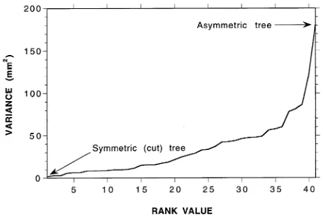
We compared variability in sap velocity in a symmetric and an asymmetric mountain ash tree by installing four sap flow loggers in each tree and examining the sap velocity fields in detail. The variance of mean sapwood thickness at breast height was estimated in a sample of 41 trees by taking 4--6 increment cores from each tree, spaced equidistantly around the bole. Based on a χ2 distribution with 40 degrees of free-dom, the mean variance was 5.2 mm2 with 99.5% confidence limits of 3.2 and 10.3 mm2. Tree 12 was the most symmetric tree, with sapwood thicknesses of 31, 32, 32 and 34 mm and a variance of 1.6 mm2. The most asymmetric tree (Tree 8) had sapwood thicknesses of 12, 20, 31 and 43 mm and a variance of 181.6 mm2. The distribution of ranked variance values for the 41 sample trees is shown in Figure 2.
For Trees 8 and 12, we examined daytime sap velocities gathered over several days of sampling. For each tree, sap velocity was determined at 20-min intervals by 16 sensors, distributed among four sap flow loggers, installed at breast height. We defined daytime values as those recorded during the diurnal period when heat pulse velocities exceeded the thresh-old sensitivity of the device (0.0155 mm s−1). In the symmetric tree, the four sensors of each of the four loggers were
im-planted at depths of 8, 13, 20 and 25 mm into the sapwood, so that the four logger estimates could be compared directly. The temporal linear correlations among the 16 sets of sap velocities were determined, resulting in a correlation matrix relating sap velocity measured by each sensor to that measured by each other sensor. Because sapwood thickness varied significantly in the asymmetric tree, the four sensors of each of the four loggers were implanted at varying depths. Because of limited availability of loggers, the sap flow measurements in the two trees were not concurrent.
The sap velocity variability within both trees was examined for the time of peak flow when sap velocity profiles across the xylem are most developed (Hatton and Vertessy 1989). For each tree, the coefficient of variation in sap velocity was estimated by Monte Carlo sampling with replacement from the original data set of 16 point estimates of sap velocity. This involved randomly sampling n = 2...15 values from the pool of 16 point estimates, and computing the coefficient of variation in the sample; whenever a value was sampled it was immedi-ately returned to the pool so each value could potentially be chosen multiple times in any given sampling run. For each sample n, the procedure was repeated 10,000 times, resulting in a statistically robust estimate of the mean coefficient of variation in sap velocity for a range of sample sizes. In the symmetric tree, we sampled sap velocities at the time of peak flow during both the pre- and post-cut periods. An analysis of variance was employed to test the null hypothesis that there were no significant differences in sap velocity among the four sampling depths in each tree or among sap flow loggers at the time of sampling.
Stand water use measurements
To determine stand water use, we related mean daily sap flow of 10 trees to scalar variables such as stem diameter and leaf area, replicating the study of Vertessy et al. (1995) that was carried out in a younger mountain ash stand. A 70 × 70 m plot, containing 94 mountain ash trees with dbh values ranging between 26.6 and 97.1 cm, with a median of 57.6 cm, was marked out. Ten sample trees were selected from the plot for detailed examination; these had dbh values ranging between 39.5 and 89.3 cm, with a median of 62.8 cm. The sample trees were thus slightly skewed toward the large end of the tree population in the plot.
Sap flow was measured over a 50-day period in the 10 sam-ple trees with five sap flow loggers. Two of the loggers were assigned to a ‘control’ tree (Tree 9) for the whole sampling period, whereas the remaining three loggers were ‘roamed’ amongst the other nine trees, usually for a 10-day period at a time. In every case, the sap flow loggers were installed at breast height. Daily sap flow totals in the control tree were regressed against simultaneously gathered values for the roaming log-gers (cf. Vertessy et al. 1995), enabling us to estimate the water use of all 10 sample trees over the entire 50-day measurement period.
Destructive sampling
After sap flow measurements were completed, each of the 10 trees was felled to permit accurate determination of height, sapwood area at breast height, and canopy leaf weight. The height and leaf mass of Tree 10 could not be sampled because it became caught up in the canopy of a neighboring tree after felling. As a replacement, Tree 11 was felled and sampled in the same manner as the other trees, though sap flow was not monitored in this tree. Tree 12 (the cut tree) was also sampled in a similar manner but the sap flow data obtained from this tree were not synchronous with the data collected for the other nine trees. Hence, a full data set is only available for nine trees. A stem disc was taken at breast height in each tree to enable accurate determination of sapwood area, based on color differ-ences. After the stem disc had been exposed to air for several days, the heartwood became brown and the sapwood remained straw colored. Sapwood thickness was measured at several points around the bole with a ruler.
Leaf weight was converted to leaf area by measuring the leaf area/leaf weight ratio of a subset of leaves from each tree. A total fresh leaf mass of 2.56 kg (sampled from 11 trees) was fed through a planimeter and yielded a leaf area of 6.25 m2. This equates to a fresh leaf area to weight ratio of 2.44 m2 kg−1, which is similar to the value of 2.41 m2 kg−1 determined by Vertessy et al. (1995) for a 15-year-old mountain ash stand.
Results
Cut tree experiment
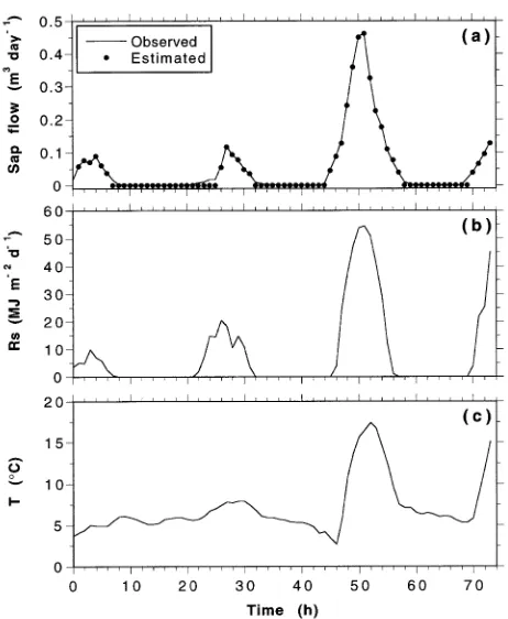
Hourly values of water loss from the reservoir over the 3-day experiment are plotted in Figure 3 along with the mean of the four hourly sap flow estimates. Hourly values of solar radiation and temperature during the experiment are also shown; unfor-tunately, the humidity sensor malfunctioned during this period. The first half of the experiment was characterized by cool and cloudy weather, whereas the second half was characterized by warm, sunny conditions. A total of 0.167 m3 of water was taken up from the reservoir, whereas the estimates from the four sap flow loggers were 0.156, 0.164, 0.162 and 0.162 m3, with a mean of 0.161 m3. All four loggers exhibited almost identical temporal patterns of sap flow. Throughout the 3-day measure-ment period, the mean hourly sap flow estimates of water uptake were virtually identical to the directly observed values of water uptake. It was only during times of low flow (at night) that the sap flow estimates were in error. Because of a lack of sensitivity in the loggers, low flows (< 0.05 m3 day−1) were recorded as no flow. This explains why the total sap flow estimates are slightly lower than the observed water uptake by the tree.
Flow variability experiment
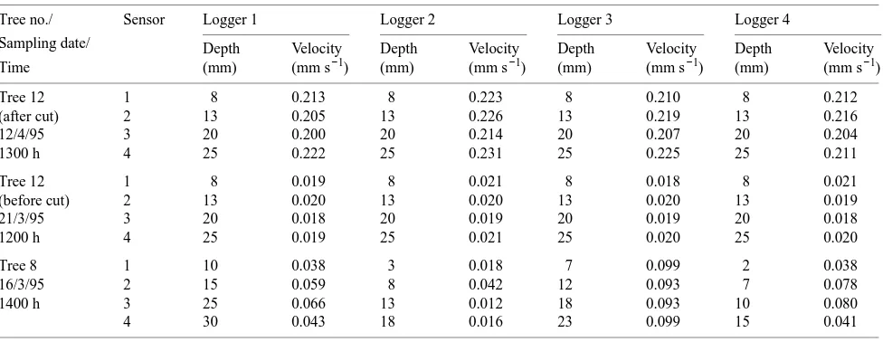
At 1300 h on April 12, the time of peak flow in the 3-day post-cut period, sap velocity recorded by the 16 sensors in the symmetric tree (Tree 12) varied between 0.200 and 0.231 mm s−1 (Table 1). At the time of peak flow, there was no significant difference in sap velocity among sapwood depths sampled or
among the loggers (ANOVA, P > 0.05). Sap velocity variabil-ity in the symmetric tree was also statistically nonsignificant (ANOVA, P > 0.05) before the cut, varying between 0.018 and 0.021 mm s−1 at the time of peak flow at 1200 h on March 21 (Table 1). Absolute sap velocity values in the symmetric tree were much lower before the cut than after the cut, partly because of weather conditions prevailing during the sampling period, but mainly because the effect of flow resistance through the root system was eliminated after the cut. In the asymmetric tree (Tree 8), there was significant variability in sap velocity amongst the 16 sensors with velocities ranging between 0.012 and 0.099 mm s−1 at the time of peak flow, 1400 h on March 16 (Table 1).
Figure 4 shows the relationships between sample size and the coefficient of variation of mean sap velocity, estimated by the Monte Carlo sampling approach, for the asymmetric tree and for the symmetric tree both before and after the cut. We compared the three curves with the relationship determined by Hatton et al. (1995) for E. populnea F.J. Muell., a semi-arid woodland species noted for its high sap velocity variability. The cut had a minimal effect on sap flow variability within the symmetric tree. Based on four sensors, the normal configura-tion per tree in our study, the coefficient of variaconfigura-tion in the symmetric tree was 2.0%, compared to 25.4% in the asymmet-ric tree. By contrast, Hatton et al. (1995) determined a coeffi-cient of variation of 31.4% (based on four sensors) in a typical E. populnea tree.
For the symmetric tree, the 128 pair-wise coefficients of determination (r2) among the 16 point estimates of sap veloc-ity (collected over 3 days after the cut) ranged between 0.83 and 0.98, with a mean of 0.94 (n = 72). In combination with the results from the sampling variability analysis, which dem-onstrated that, on average, sensors placed throughout the sap-wood yielded similar estimates of sap velocity at peak flow, these results indicate that sap velocity was uniform throughout the xylem of the symmetric tree during the day. This was clearly not the case in the asymmetric tree.
Destructive sampling
Measurements of tree diameter, height, sapwood area and leaf area for each of the sample trees are listed in Table 2. Tree heights varied between 44 and 65 m, leaf areas varied between 45.1 and 404.8 m2, and sapwood areas varied between 209 and 843 cm2.
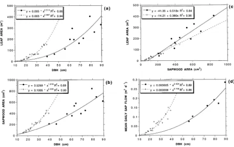
Observed relationships between stem diameter, leaf area and sapwood area are shown in Figure 5, relative to similar
rela-tionships reported for 15-year-old mountain ash trees by Vertessy et al. (1995). Power function-based regressions indi-cated that stem diameter explained 66% and 69% of the vari-ation in leaf area and sapwood area, respectively. A simple linear regression indicated that sapwood area explained 84% of the variation in leaf area. Although these correlations were not as strong as those reported by Vertessy et al. (1995) for 15-year-old mountain ash trees, they were all statistically sig-nificant at the 0.001 level, according to the two-tailed signifi-cance test for correlation coefficients (Rosner 1990).
Application of the equation shown in Figure 5a to the stem diameter census for all 94 trees in the 70 × 70 m plot yielded an estimate of the total leaf area of the plot of 13,980 m2, which is equivalent to an LAI of 2.85. This LAI is lower than normal for mountain ash forests of this age class (Watson and Vertessy 1996), probably because of the ridge-top position of the site, which is characterized by higher insolation and drier soil conditions than is typical for such forests. We also estimated the plot LAI independently with an LAI-2000 Plant Canopy Analyzer (Li-Cor Inc., Lincoln, NE) (Welles and Norman 1991), and obtained a value of 2.6.
Sap flow measurements
Sap flow in the control tree (Tree 9) varied considerably over the 50-day measurement period, fluctuating between 0.061 and 0.323 m3 day−1, averaging 0.172 m3 day−1, and totaling 8.601 m3 (Figure 6). Over the first 15 days of the experiment, because conditions were cool and overcast, sap flow rates were low, averaging about 0.1 m3 day−1. Warmer and clearer condi-tions prevailed over the next 20 days and sap flows of 0.3 m3 day−1 were attained on several days. The last 15 days of the experiment were characterized by mainly overcast and cooler conditions, and sap flow declined accordingly.
Daily sap flow values in the control tree (Tree 9) correlated well with simultaneously measured values in Trees 3, 6, 7, 8 and 11; the coefficients of determination (r2) varied between 0.66 and 0.99 (Table 3). Daily sap flow in Tree 2 was weakly
Table 1. Variation in peak sap velocities within the most symmetric tree (Tree 12) before and after the cut, and within the most asymmetric tree (Tree 8).
Tree no./ Sensor Logger 1 Logger 2 Logger 3 Logger 4
Sampling date/ Depth Velocity Depth Velocity Depth Velocity Depth Velocity
Time (mm) (mm s−1) (mm) (mm s−1) (mm) (mm s−1) (mm) (mm s−1)
Tree 12 1 8 0.213 8 0.223 8 0.210 8 0.212
(after cut) 2 13 0.205 13 0.226 13 0.219 13 0.216
12/4/95 3 20 0.200 20 0.214 20 0.207 20 0.204
1300 h 4 25 0.222 25 0.231 25 0.225 25 0.211
Tree 12 1 8 0.019 8 0.021 8 0.018 8 0.021
(before cut) 2 13 0.020 13 0.020 13 0.020 13 0.019
21/3/95 3 20 0.018 20 0.019 20 0.019 20 0.018
1200 h 4 25 0.019 25 0.021 25 0.020 25 0.020
Tree 8 1 10 0.038 3 0.018 7 0.099 2 0.038
16/3/95 2 15 0.059 8 0.042 12 0.093 7 0.078
1400 h 3 25 0.066 13 0.012 18 0.093 10 0.080
4 30 0.043 18 0.016 23 0.099 15 0.041
but significantly (P = 0.05) correlated with that in the control tree; however, we rejected the data from Tree 2 because the sap flow rates appeared anomalously high in relation to the leaf area of the tree (i.e., more than twice that of the other trees). Correlations between daily sap flow in the control tree (Tree 9)
and Trees 1, 4 and 5 were poor and not statistically significant at the 0.05 level, probably because of poor probe implantation in these three trees. For this reason we did not estimate 50-day sap flow totals for these three trees. Water use was not meas-ured in Tree 10, and measurements of water use of the cut tree
Table 2. Stem diameter, height, sapwood area, leaf area, sap velocity and sap flow for the 12 sample trees at Black Spur. A dash denotes a value that could not be computed.
Tree Diameter Height Sapwood Leaf Mean daily Mean daily Min. daily Max. daily Total sap
(cm) (m) area area sap velocity sap flow sap flow sap flow flow
(cm2) (m2) (mm s−1) (m3 day−1) (m3 day−1) (m3 day−1) (m3)
1 60.6 55.8 357 197.8 -- -- -- --
2 39.5 44.1 213 45.1 -- -- -- --
3 79.2 60.0 843 404.8 0.026 0.191 0.077 0.328 9.54
4 62.8 57.7 534 296.5 -- -- -- --
5 64.3 56.7 579 195.8 -- -- -- --
6 56.0 54.3 390 111.3 0.022 0.075 0.042 0.123 3.77
7 89.3 57.6 618 330.4 0.053 0.285 0.091 0.553 14.25
8 73.0 51.8 452 206.8 0.041 0.159 0.060 0.263 7.96
9 83.3 54.9 695 263.5 0.029 0.172 0.061 0.323 8.60
10 46.2 49.6 209 66.1 -- -- -- --
--11 59.5 -- 403 -- 0.029 0.103 0.042 0.160 5.13
12 69.0 65.0 396 163.0 -- -- -- --
(Tree 12) was made over a different period than those of the other trees. Hence, 50-day sap flow statistics were only com-piled for six of the 12 sample trees.
Mean daily sap flow over the 50-day period varied between 0.075 m3 day−1 (Tree 6) and 0.285 m3 day−1 (Tree 7) (Table 2). Stem diameter explained 89% of the variation in mean daily sap flow values in Trees 3, 6, 7, 8, 9 and 11 (Figure 5d), which is slightly higher than observed for young mountain ash trees by Vertessy et al. (1995). For n = 6, an r2 value of 0.89 is statistically significant at the 0.001 level (Rosner 1990). Mean sap velocity in these trees varied between 0.022 and 0.053 mm s−1, and averaged 0.033 mm s−1.
Stand water use estimates
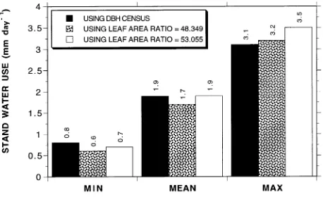
Two methods were used to extrapolate our estimates of daily sap flow in individual trees to an areal basis. In Method 1, we took the relationship between stem diameter and mean daily sap flow (Figure 5d) and applied this to the measured dbh of all 94 trees in the 70 × 70 m plot. This calculation was repeated for minimum and maximum sap flow values; earlier analyses indicated that stem diameter explained 84 and 91% of the variation in minimum and maximum sap flow rates, respec-tively. In Method 2, we related the leaf area of a ‘reference tree’ (Tree 9) to the Plant Canopy Analyzer estimate of the plot LAI (2.6). Multiplying the LAI by the plot area of 4,900 m2 yielded a total leaf area for the plot of 12,740 m2. Dividing the total leaf
area of the plot by the leaf area of the reference tree (263.5 m2) gave a value of 48.349, which we refer to as the ‘leaf area ratio.’ The mean, minimum and maximum daily sap flow values for the ‘reference tree’ were multiplied by the leaf area ratio to calculate the mean, minimum and maximum transpiration rates for the whole plot. This method assumes that there is a linear correlation between leaf area and sap flow in the stand. This is probably valid for stands with LAI values of 3 or less; beyond this value, self-shading and shading by adjacent trees would tend to break down the relationship (Waring and Sil-vester 1994). Although Yoder et al. (1994) and Mencuccini and Grace (1996) showed that the relationship was not always linear across age gradients of particular forest types, Vertessy et al. (1995) demonstrated linearity across a broad tree size gradient in a young even-aged mountain ash forest. Linearity was also observed in Pinus radiata D. Don trees of various sizes by Teskey and Sheriff (1996).
Estimates, by the two methods, of minimum, mean and maximum daily water use of all 94 trees in the plot are com-pared in Figure 7. Based on stem diameter as the scalar (Method 1), the estimated values were 0.8, 1.9 and 3.1 mm day−1, respectively. Based on leaf area ratio as the scalar (Method 2), the estimated values were 0.6, 1.7 and 3.2 mm day−1, respectively. If a plot LAI of 2.85 was assumed (as computed by the equation in Figure 5a), the leaf area ratio increased to 53.055, and the minimum, mean and maximum daily water use estimates increased to 0.7, 1.9 and 3.5 mm day−1, respectively. Total water use by the mountain ash trees in the plot over the 50 days of sampling was estimated to be 95 mm by Method 1, and 85 or 95 mm by Method 2, depending on which leaf area ratio value was used.
Discussion
Cut tree experiments have been used by several workers to validate sap flow estimates of eucalypt tree water use. Doley and Grieve (1966) applied an early version of the sap flow method (based on surface heating of the stem) to several small E. marginata J. Donn. ex Sm. Jarrah. trees and found that sap flow estimates equated to about half the actual tree water uptake. In an application of the technique to several E. regnans
Figure 6. Variation in total daily sap flow in the control tree (Tree 9) over the 50-day sampling period.
Table 3. Coefficients of determination (r2) for daily sap flow in nine mountain ash trees, relative to the control tree (Tree 9). The letter n denotes the number of simultaneous days of recording. No simultane-ous water use data were available for Trees 10 and 12.
Tree r2 n F statistic
1 0.24 15 0.05 < P < 0.1
2 0.39 13 0.01 < P < 0.05
3 0.66 15 P < 0.001
4 0.31 12 0.05 < P < 0.1
5 0.06 6 P > 0.01
6 0.98 9 P < 0.001
7 0.99 9 P < 0.001
8 0.83 4 0.05 < P < 0.1
11 0.93 24 P < 0.001
saplings, Dunn and Connor (1993) obtained sap flow estimates that were within 5% of actual tree water use. Hatton et al. (1995) reported a 15% difference between estimated and ac-tual water use in an E. populnea tree, and Barrett et al. (1995) reported differences of 1--11% in their study examining sap flow behavior in two small E. maculata Hook. trees. Each of these studies was performed on small saplings and lasted less than 24 h in duration.
Olbrich (1991) applied the in situ cut tree technique to a 56-m-tall E. grandis W. Hill ex Maiden. with similar leaf area (219 m2) and sapwood area (371 cm2) to our cut tree and found that the sap flow estimate of water uptake was about 12% greater than the actual value. Because Olbrich (1991) attrib-uted part of the discrepancy to the use of a flexible reservoir to hold water around the stem, we used a rigid storage system in our study. We found that the sap flow method underestimated cumulative water uptake over 3 days by less than 4%. Esti-mated sap flow closely tracked actual water uptake throughout the measurement period, except for periods of very low uptake (< 0.05 m3 day−1) when the sap flow logger recorded no flow. We conclude that the sap flow method is a valid means of determining the water use behavior of a single mountain ash tree, although the sensitivity of the sap flow sensor needs to be improved if accurate estimates of low sap flows are required.
We sampled the variability in sap velocities in one symmet-rical and one asymmetsymmet-rical tree and found that the degree of variability in sap velocity within mountain ash trees appears to be a reflection of the degree of symmetry in sapwood thick-ness. In the symmetrical tree, sap velocity was fairly uniform throughout the xylem (both before and after the cut), indicating that sap flow could be estimated accurately with a single logger equipped with four sensors. By contrast, Olbrich (1991) con-cluded that at least eight sampling points were needed in E. grandis trees larger than 20 cm in diameter, and Hatton et al. (1995) argued that even greater sampling resources were re-quired to estimate sap flow accurately in a single E. populnea tree. The high degree of variability in sap velocity in our asymmetrical mountain ash tree would also necessitate more than four sampling points. However, mountain ash trees with highly asymmetrical sapwood cross sections make up only a small part of the mountain ash forest resource (Figure 2) and can be easily avoided in field sampling programs. We suggest that it is desirable to allocate sap flow logger resources across as many trees as possible because sap velocity variability was much greater among trees than within trees. For example, there was less variation within the symmetrical tree than among the six trees for which we have measurements of mean sap veloc-ity (cf. Tables 1 and 2). Granier et al. (1996) also concluded that sap velocity variability among trees in a stand was nor-mally much greater than sap velocity variability within indi-vidual trees.
Several studies have documented strong relationships be-tween allometric properties of trees and tree water use (Hatton and Wu 1995, Teskey and Sheriff 1996). We confirmed the earlier observations of Vertessy et al. (1995) that stem diameter is a good predictor of sapwood area, leaf area and mean daily sap flow in mountain ash trees. Although the associations
between these variables were not as strong as previously noted for young (15-year-old) stands, they were statistically signifi-cant at the 0.001 level. As the forest ages, sapwood area becomes a progressively smaller and more variable fraction of basal area; hence, several workers have advocated using sap-wood area rather than stem diameter as the prime scalar for leaf area and therefore tree water use prediction (Waring et al. 1977, Whitehead 1978, Waring 1983). However, it is more practical to use stem diameter than sapwood area as the prime scalar for stand-level predictions of leaf area and tree water use in mature mountain ash forests because sapwood area is diffi-cult to measure. For instance, Vertessy et al. (1995) determined that three or more cores (sometimes as many as 10) were required to estimate sapwood thickness within 5 mm of the true mean with 95% confidence in young mountain ash trees. It is probable that even more estimates would be needed for older mountain ash trees to obtain similar accuracy. Waring (1983) has pointed out that, for older trees, sapwood area at the base of the live crown is a better scalar than sapwood area at breast height, necessitating the calculation of taper coefficients for older trees, and hence more work and possibly greater uncertainty. Another advantage of using stem diameter as the primary scalar for leaf area and sap flow estimations is that many stem diameter and stocking rate data are available in forest inventories gathered by forest agencies.
A major obstacle to overcome with respect to scaling indi-vidual tree water use to the stand level is that separate stem diameter--leaf area relationships are needed for mountain ash stands of different ages. For instance, based on the equation reported by Vertessy et al. (1995) for 15-year-old mountain ash (shown in Figure 5a), the predicted LAI of the Black Spur site would be 12.9, whereas a value of 2.85 was obtained based on the equation derived in this study (also shown in Figure 5a), and the Plant Canopy Analyzer-based estimate was 2.6. A composite equation fitted to both the Vertessy et al. (1995) data and the data from this study (leaf area = 0.127dbh1.797, n = 29, r2 = 0.82) yielded a plot LAI of 3.7. Watson and Vertessy (1996) have recently developed a general empirical model that uses stem diameter data to predict leaf area values for moun-tain ash stands of any age; however, similar, generalized rela-tionships that relate stem diameter and sapwood area and sap flow have yet to be developed for mountain ash stands.
accuracy by the Plant Canopy Analyzer measurement tech-nique.
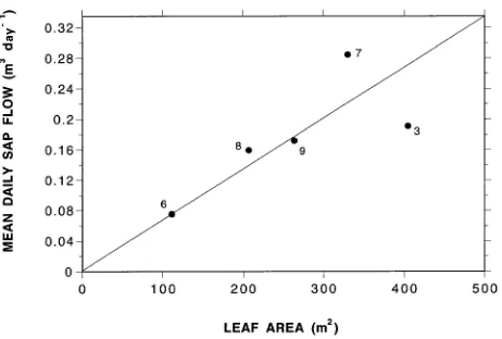
Although Method 1 is more onerous to apply, it yields more robust estimates of stand water use than Method 2. The mean daily plot water use calculated by Method 2 was 11% lower than the value computed by Method 1. However, there was no difference between the two methods when we applied the leaf area ratio based on the destructive sampling estimate of plot LAI (2.85). Method 2 is strongly influenced by the ‘typicality’ of the reference tree and the accuracy of the plot LAI estimate. For Method 2 to yield an estimate close to Method 1, the reference tree needs to lie close to the line of best fit in the sap flow--leaf area relationship (Figure 8). Tree 9 was used as the reference tree in the leaf area ratio scaling method (Method 2) because it was the sap flow measurement control tree. Had Tree 3 been used as the reference tree then the estimates of the two methods would not have been so close.
The mean daily sap velocity and stand water use estimates obtained for the Black Spur site compare closely with those observed in other studies of mountain ash forest water use over spring--summer periods. Our mean daily sap velocity of 0.033 mm s−1 is similar to that reported by Vertessy et al. (1995) for a 15-year-old mountain ash forest, and similar to the value of 0.032 mm s−1 obtained for a 50-year-old mountain ash stand by Dunn and Connor (1993). These data support the notion that the stand mean of daily sap velocity (averaged for a month or more over spring--summer) does not vary signifi-cantly among mountain ash stands of different ages. We con-clude that reasonable calculations of stand water use can be made for different age classes of mountain ash if a reliable stand age--sapwood area relationship can be developed. Our mean daily stand water use estimate for the Black Spur site (1.9 mm; based on scaling Method 1) is slightly lower than the 2.3 mm observed by Vertessy et al. (1995) for a 39-day spring sampling period in a young mountain ash forest. We conclude that long-term sap flow measurements in mountain ash forests are needed to determine how climate factors affect stand water use throughout the year.
Acknowledgments
This study was funded by the Cooperative Research Center for Catch-ment Hydrology. Jim Brophy and Jamie Margules helped out with many aspects of the field experiments. We also thank Melbourne Water and the Victorian Department of Conservation and Environment for valuable field assistance. Drs. J. Landsberg and R. Waring kindly provided valuable suggestions on a draft of this paper.
References
Barrett, D.J., T.J. Hatton, J.E. Ash and M.C. Ball. 1995. Evaluation of the heat pulse velocity technique for measurement of sap flow in rainforest and eucalypt forest species of south-eastern Australia. Plant Cell Environ. 18:463--469.
Davis, S., R.A. Vertessy, D.L. Dunkerley and R.G. Mein. 1996. The influence of scale on the measurement of saturated hydraulic con-ductivity in a forest soil. Australian Institute of Engineers, Hydrol-ogy and Water Resources Symp. National Conference Publication No. 96/05, Canberra, pp 103--108.
Doley, D. and B.J. Grieve. 1966. Measurement of sap flow in a eucalypt by thermo-electric methods. Aust. For. Res. 2:3--27. Dunn, G.M. and D.J. Connor. 1993. An analysis of sap flow in
mountain ash (Eucalyptus regnans) forests of different age. Tree Physiol. 13:321--336.
Edwards, W.R.N., P. Becker and J. Èermak. 1997. A unified nomen-clature for sap flow measurements. Tree Physiol. 17:65--67. Granier, A., P. Biron, N. Bréda, J.Y. Pontailler and B. Saugier. 1996.
Transpiration of trees and forest stands: short and long-term moni-toring using sapflow methods. Global Change Biol. 2:265--274. Hatton, T.J. and R.A. Vertessy. 1989. Variability of sapflow in a Pinus
radiata plantation and the robust estimation of transpiration.
Aus-tralian Institute of Engineers, Hydrology and Water Resources Symp., National Conference Publication No. 89/19, Canberra, pp 6--10.
Hatton, T.J. and H.I. Wu. 1995. Scaling theory to extrapolate individ-ual tree water use to stand water use. Hydrol. Processes 9:527--540. Hatton, T.J., S.J. Moore and P.H. Reece. 1995. Estimating stand transpiration in Eucalyptus populnea woodland with the heat pulse method: method errors and sampling strategies. Tree Physiol. 4:219--227.
Jayasuriya, M.D.A., G. Dunn, R. Benyon and P.J. O’Shaughnessy. 1993. Some factors affecting water yield from mountain ash
(Euca-lyptus regnans) dominated forests in south-east Australia. J. Hydrol.
150:345--367.
Kuczera, G.A. 1987. Prediction of water yield reductions following a bushfire in ash-mixed species eucalypt forest. J. Hydrol. 94:215--236. Landsberg, J.J., T.W. Blanchard and B. Warrit. 1976. Studies on the movement of water through apple trees. J. Exp. Bot. 27:579--596. Langford, K.J. 1976. Change in yield of water following a bushfire in
a forest of Eucalyptus regnans. J. Hydrol. 29:87--114.
Langford, K.J. and P.J. O’Shaughnessy. 1977. First progress report, North Maroondah. Melbourne and Metropolitan Board of Works, Catchment Hydrology Research Report Number MMBW-W-0005, Melbourne, Australia, 340 p.
Mencuccini, M. and J. Grace. 1996. Hydraulic conductance, light interception and needle nutrient concentration in Scots pine stands and their relations with net primary productivity. Tree Physiol. 16:459--468.
Olbrich, B.W. 1991. The verification of the heat pulse velocity tech-nique for measuring sap flow in Eucalyptus grandis. Can. J. For. Res. 21:836--841.
Roberts, J. 1977. The use of tree-cutting in the study of the water relations of mature Pinus sylvestris L. J. Exp. Bot. 28:751--767. Figure 8. Observed relationship between leaf area and mean daily sap
Rosner, B.A. 1990. Fundamentals of biostatistics, 3rd Edn. PWS-Kent Publishing, Boston, 655 p.
Teskey, R.O. and D.W. Sheriff. 1996. Water use by Pinus radiata trees in a plantation. Tree Physiol. 16:273--279.
Vertessy, R., R. Benyon and S. Haydon. 1994. Melbourne’s forest catchments: effect of age on water yield. Water 21:17--20. Vertessy, R.A., R.G. Benyon, S.K. O’Sullivan and P.R. Gribben. 1995.
Relationship between stem diameter, sapwood area, leaf area and transpiration in a young mountain ash forest. Tree Physiol. 15:559--568.
Waring, R.H. 1983. Estimating forest growth and efficiency in relation to canopy leaf area. Adv. Ecol. Res. 13:327--354.
Waring, R.H. and W.B. Silvester. 1994. Variation in foliar δ13C values within the crowns of Pinus radiata trees. Tree Physiol.
14:1203--1213.
Waring, R.H., H.L. Gholz, C.C. Grier and M.L. Plummer. 1977. Evaluating stem conducting tissue as an estimator of leaf area in four woody angiosperms. Can. J. Bot. 55:1474--1477.
Watson, F.G.R. and R.A. Vertessy. 1996. Estimating leaf area index from stem diameter measurements in mountain ash forest. Coop-erative Research Centre for Catchment Hydrology, Technical Re-port 96/7, Canberra, Australia, 102 p.
Welles, J.M. and J.M. Norman. 1991. Instrument for indirect measure-ment of canopy architecture. Agron. J. 83:818--825.
Whitehead, D. 1978. The estimation of foliage area from sapwood basal area in Scots pine. Forestry 51:35--47.