The Significance of Spatial Reconstruction in Finite
Volume Methods for the Shallow Water Equations
Noor Hidayat
Faculty of Science and Technology, Airlangga University, Surabaya, Indonesia; and Department of Mathematics, Brawijaya University, Malang, Indonesia
Suhariningsih
Department of Physics, Airlangga University, Surabaya, Indonesia
Agus Suryanto
Department of Mathematics, Brawijaya University, Malang, Indonesia
Sudi Mungkasi
Department of Mathematics, Sanata Dharma University, Yogyakarta, Indonesia
Copyright © 2014 Noor Hidayat, Suhariningsih, Agus Suryanto and Sudi Mungkasi. This is an open access article distributed under the Creative Commons Attribution License, which permits unrestricted use, distribution, and reproduction in any medium, provided the original work is properly cited.
Abstract
Keywords: spatial reconstruction, finite volume, shallow water equations
1 Introduction
The free surface, unsteady water flow is modeled by the well-known Saint-Venant equations. This model is also called the shallow water (wave) equations. Accurately solving these equations is important, because it can help simulations of natural events, such as floods, tsunamis, dam breaks, tides, etc. To get numerical solutions of these equations, there are many numerical methods available in the literatures [8, 9, 12, 15], for examples finite difference and finite volume methods. Finite difference methods are based on the differential form of the equations. They may lead to some difficulties when we want to resolve discontinuities, because differential equations assume that solutions are smooth. In contrast, finite volume methods are based on the integral form of the equations. Integral equations do not assume smoothness of their solutions, and hence finite volume methods are able to resolve smooth and nonsmooth solutions (see [2, 6, 7, 8, 13]). However the accuracy of those numerical methods will be dependent on the integration with respect to both time (temporal) and space (spatial).
In this paper we investigate the significance of spatial reconstruction in finite volume methods when solving the shallow water equations. We show that a higher order reconstruction of the spatial domain can improve the accuracy of the numerical methods. To do so we use one type of temporal integration. We then compare the performance of two types (that is, constant and linear) of spatial reconstructions.
This paper is organized as follows. Shallow water equations are recalled in Section 2. We present the finite volume method that we use to solve the shallow water equations in Section 3. Numerical results are presented in Section 4. We draw some concluding remarks in Section 5.
2 Shallow Water Equations
We consider the following one dimensional shallow water equations
(1)
( ) (2)
where denotes the time variable, denotes the space variable, is
water height or depth, is velocity, represents the bottom
elevation or topography, and is the acceleration due to gravity. The absolute
water level (stage) is defined as . Equations (1) and (2)
(3)
We refer to [5] for these forms of shallow water equations.
3 Finite Volume Methods
In this section, we recall a finite volume method proposed in [5, 7], which was developed for steady state problems. The finite volume method can then be used to solve steady and unsteady state problems. Here we assume that the space
is discretized into a finite number of cells uniformly with cell width and that
time is also discretized uniformly with size of time step is . Then equation (3)
can be solved using the finite volume method
Here subscript represents the th cell and superscript denotes the time level
at . This means is the right vertex of the th cell. The
variable is an approximation of the analytical source
At a vertex of a cell, we use approximations for both sides
,
(8)
in which the superscript “-” is for the left side approximation and the superscript “+” is for the right side approximation of that vertex. Both approximations at left and right sides of the vertex is obtained from polynomial reconstructions
∑ , (9)
where is a polynomial supported on the interval [ ] which is
centered at the midpoint , and is defined at time , is the
polynomials. Let the linear functions are
( )
(10)
where is the slope. This slope must be chosen with care so that numerical
solutions of the shallow water equations are non oscillatory. This requires that the value of the slope must be limited. A well-known type of that limiter is the minmod slope. The minmod limiter was used by a number of authors for their work, such as in [1, 4, 5, 10, 11, 16]. In this paper, we use the following minmod limiter as in [5]:
(
) , (11)
where (sgn( )+sgn( ) ) | | | | . Note that if for
all , then the space discretization becomes first order.
In order that the finite volume method is able to solve the steady state problems (as well as unsteady state problems), we use the central semi discrete
scheme. Here we implement a numerical flux, as in [7] and numerical
source terms, ̅ , as given in [5]. This scheme is then
̅ (12)
where
( ) ( ) [ ]
and ̅ ( ̅
̅ ). Here ̅
and
̅
.
(13)
For simplicity, we apply the forward Euler method to solve equation (12).
4 Numerical Results
(a) the steady state of a lake at rest, (b) the steady state of moving water and (c) an unsteady state of dam break problem. We compare the results of first order discretization in space (Method I) and those of second order spatial discretization (Method II).
Our numerical setting is as follows. We test the finite volume method for
the following three cases using the uniform cells. The number of cells ( are
chosen to be 100, 200, 400, 800, 1600, 3200. For the time step, we take uniform
. We calculate the numerical error and the convergence rate. To
quantify numerical errors , we use the absolute error
∑ | | (14)
where and are the exact and numerical solution at , respectively. To
compute the convergence rate, we use the following formula [14]
Rate
Therefore, any omitted units should be noted to have SI units.
(a). The steady state of a lake at rest
The test of a lake at rest problem is intended to see if the above finite volume method is able to resolve the steady state of still water. We follow the test presented in [3]. Consider a lake with 1500 m of length. At the downstream boundary the water level is imposed to be 12 m and at the upstream there is no discharge. The initial condition is water at rest at the level of 12 m. The analytical solution is obviously
water at rest: discharge and flow velocity are zero,
flat free surface: water level stays at the initial level of 12 m.
We consider the geometry as given in Figure 1 and the complete description of this geometry (see [3]) is given in the following Table 1.
Figure 1. The geometry profile of the lake at rest.
Figure 2. Stage, momentum and velocity of lake at rest problem by Method I. Here we use 400 cells and final time 10 seconds.
We confirm that both methods are well-balanced, that is, the steady state of the lake at rest is preserved up to discrete level, see Figure 2 for the stage, momentum and velocity produced by Method I. We note that for that scale, Method II generates the same plots. These results are calculated using 400 cells with final time 10 seconds.
(b). The steady state of moving water over a bump
This test of steady flow over a bump is intended to verify if the numerical
0 100 200 300 400 500 600 700 800 900 1000 1100 1200 1300 1400 1500 0
Stage of lake at rest at time t=10.00
w
0 500 1000 1500
-1 0
1x 10
-13 Momentum of lake at rest at time t=10.00
Q
-14 Velocity of lake at rest at time t=10.00
Position
method can resolve the steady state of moving water. We use the following data geometry [3]. The channel length is 25 m (meter) and the bottom equation is
{ (17)
The boundary and initial conditions are as follow. At downstream, the water level is imposed to be 2 m. At upstream, the water discharge is imposed to be 4.42
m3/s (s= second). Initially, we have a constant water level which is equal to the level
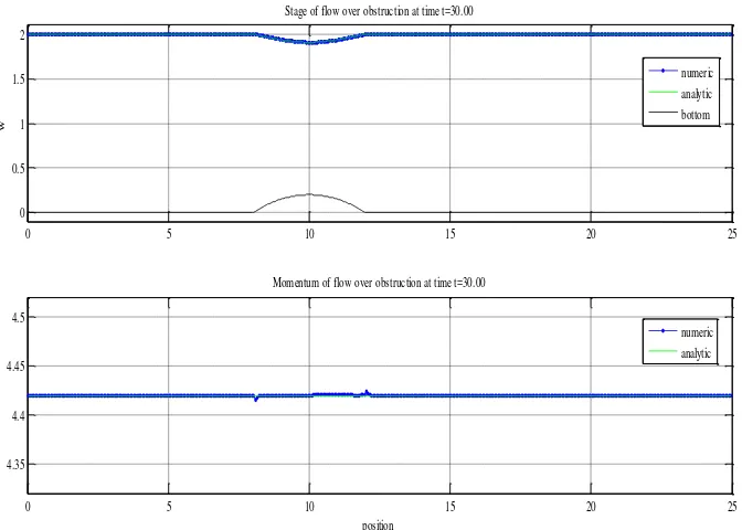
imposed downstream with discharge equals to zero. The stage, momentum and velocity obtained by Method II at final time 30 seconds are plotted in Figure 2. It is seen that the numerical solutions agree very well with the exact solution. We note that Method I also generates the same plot. However, detail analysis shows that Method II has much better accuracy as shown in Table 2.
Figure 3. Stage and momentum on flow of obstruction by Method II. Here we use 400 cells and final time 30 seconds.
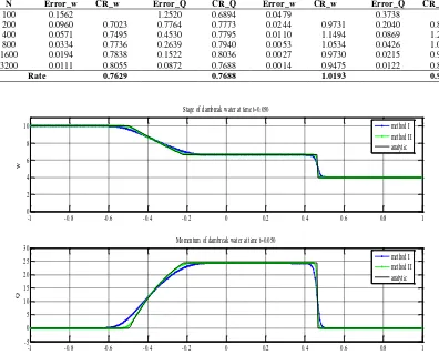
Table 2. The error of obstruction problems by Method I and II.
Method I Method II 1600 3.9488e-004 0.9919 8.2664e-004 0.9527 1.1855e-004 1.0328 8.5320e-006 1.9948
Rate 0.9366 0.9063 Rate 1.0996 1.9682
(c). An unsteady state of dam break problem
The dam break problem is intended to test if the numerical method can
0 5 10 15 20 25
Stage of flow over obstruction at time t=30.00
w
Momentum of flow over obstruction at time t=30.00
resolve unsteady flows. The topography is given by a horizontal bottom
where . The initial water height is given by
{
(18)
The analytical solution of this problem has been found in [17] and extended in [13]. The simulation results using 400 cells and final time 0.05 seconds are shown in Table 3 for errors and Figure 4 for stage and momentum. It is seen from Table 3 that Method II gives more accurate results and higher convergence rate.
Table 3. Error of dam-break problems by Method I and II.
Method I Method II
Figure 4. Stage and momentum on simulation of dam-break problem by Method I and II. Here we use 400 cells and final time 0.05 seconds.
5 Conclusions
The influence of spatial reconstruction in finite volume methods when solving the shallow water equations has been investigated. The constant reconstruction for the space domain is simple and cheap to compute. However, we
-1 -0.8 -0.6 -0.4 -0.2 0 0.2 0.4 0.6 0.8 1
Stage of dambreak water at time t=0.050
w
Momentum of dambreak water at time t=0.050
find that linear reconstruction of the space domain has a great improvement to the accuracy of the methods. We conclude that the accuracy of the spatial reconstruction has a significant role in the accuracy of the numerical methods.
Acknowledgements. Part of this work was supported by Program Hibah Kompetisi of the Department of Mathematics, Brawijaya University, funded by the General Directorate of Higher Education, Indonesia.
References
[1] F. Bianco, G. Puppo and G. Russo, High order central schemes for hyperbolic
system of conservation laws, SIAM Journal on Scientific Computing, 21
(1999), 294–322.
[2] F. Bouchut, Nonlinear stability of finite volume methods for hyperbolic
conservation laws and well-balanced schemes for sources, Birkhauser,
Bassel, 2004.
[3] N. Goutal and F. Maurel, Momentum equation source term calculation &
steady state validation, Proceedings of the 2nd Workshop on Dam-Break Wave
Simulation, No. HE-43/97/016/B, Departement Laboratoire National
d’Hydraulique, Groupe Hydraulique Fluviale, Electricite de France, Chatou,
1997.
[4] A. Harten, High resolution schemes for hyperbolic conservation laws. Jurnal
of Computational Physics,135 (1997), 260–278.
[5] A. Kurganov and D. Levy, Central-upwind schemes for the Saint-Venant
system, ESAIM: Mathematical Modelling and Numerical Analysis,36 (2002),
397–425.
[6] A. Kurganov, S. Noelle and G. Petrova, Semidiscrete central-upwind schemes
for hyperbolic conservation laws and Hamilton–Jacobi equations. SIAM
Journal on Scientific Computing, 23 (2001), 707–740.
[7] A. Kurganov and E. Tadmor, New high-resolution central scheme for
non-linier conservation laws and convection-diffusion equations, Journal of
Computational Physics,160 (2000), 241–282.
[8] R. J. LeVeque, Numerical methods for conservation laws, 2nd Edition,
[9] R. J. LeVeque, Finite-volume methods for hyperbolic problems, Cambridge University Press, Cambridge, 2004.
[10] D. Levy, G. Puppo and G. Russo, Central WENO schemes for hyperbolic
systems of conservation laws, ESAIM: Mathematical Modelling and
Numerical Analysis,33 (1999), 547–571.
[11] X.D. Liu and E. Tadmor, Third order nonoscillatory central scheme for
hyperbolic conservation laws, Numerische Mathematik,79 (1998), 397–425.
[12] S. Mungkasi, A Study of well-balanced finite volume methods and refinement
indicators for the shallow water equations, Thesis of Doctor of Philosophy,
The Australian National University, Canberra, 2012.
[13] S. Mungkasi and S. G. Roberts, Analytical solution involving shock waves for
testing debris avalanche numerical models, Pure and Applied Geophysics,169
(2012), 187–1858.
[14] R. Naidoo and S. Baboolal, Application of the Kurganov-Levy semidiscrete
numerical scheme to hyperbolic problems with non-linear source term. Future
Generatian Computer System,20 (2004), 465–473.
[15] H. Nessyahu and E. Tadmor, Non-oscillatory central differencing for
hyperbolic conservation laws, Journal of Computational Physics, 87 (1990),
408–463.
[16] S. Osher and E. Tadmor, On the convergence of difference approximation to
scalar conservation laws, Mathematics of Computation,50 (1988), 19–51.
[17] J. J. Stoker, Water Waves: The Mathematical Theory with Application,
Interscience Publishers, New York, 1957.