Volume 7: OGC CDB Data Model Guidance Formerly An A Volume Part 2DB-model-guidance

(1)

Open Geospatial Consortium

Submission Date: 2016-02-22 Approval Date: 2016-09-23 Publication Date: 2017-02-23 External identifier: http://www.opengis.net/doc/BP/CDB-model-guidance/1.0

Internal reference number of this OGC® document: 16-010r3 Version: 1.0 Category: OGC® Best Practice

Editor: Carl Reed

Volume 7: OGC CDB Data Model Guidance

Formerly Annex A Volume Part 2

Copyright notice

To obtain additional rights of use, visit http://www.opengeospatial.org/legal/.

Warning

This document defines an OGC Best Practices on a particular technology or approach related to an OGC standard. This document is not an OGC Standard and may not be referred to as an OGC Standard. It is subject to change without notice. However, this document is an official position of the OGC membership on this particular technology topic.

Document type: OGC® Best Practice Document subtype: Volume 7

(2)

License Agreement

Permission is hereby granted by the Open Geospatial Consortium, ("Licensor"), free of charge and subject to the terms set forth below, to any person obtaining a copy of this Intellectual Property and any associated documentation, to deal in the Intellectual Property without restriction (except as set forth below), including without limitation the rights to implement, use, copy, modify, merge, publish, distribute, and/or sublicense copies of the Intellectual Property, and to permit persons to whom the Intellectual Property is furnished to do so, provided that all copyright notices on the intellectual property are retained intact and that each person to whom the Intellectual Property is furnished agrees to the terms of this Agreement.

If you modify the Intellectual Property, all copies of the modified Intellectual Property must include, in addition to the above copyright notice, a notice that the Intellectual Property includes modifications that have not been approved or adopted by LICENSOR.

THIS LICENSE IS A COPYRIGHT LICENSE ONLY, AND DOES NOT CONVEY ANY RIGHTS UNDER ANY PATENTS THAT MAY BE IN FORCE ANYWHERE IN THE WORLD.

THE INTELLECTUAL PROPERTY IS PROVIDED "AS IS", WITHOUT WARRANTY OF ANY KIND, EXPRESS OR IMPLIED, INCLUDING BUT NOT LIMITED TO THE WARRANTIES OF MERCHANTABILITY, FITNESS FOR A PARTICULAR PURPOSE, AND NONINFRINGEMENT OF THIRD PARTY RIGHTS. THE COPYRIGHT HOLDER OR HOLDERS INCLUDED IN THIS NOTICE DO NOT WARRANT THAT THE FUNCTIONS CONTAINED IN THE INTELLECTUAL PROPERTY WILL MEET YOUR REQUIREMENTS OR THAT THE OPERATION OF THE INTELLECTUAL PROPERTY WILL BE

UNINTERRUPTED OR ERROR FREE. ANY USE OF THE INTELLECTUAL PROPERTY SHALL BE MADE ENTIRELY AT THE USER’S OWN RISK. IN NO EVENT SHALL THE COPYRIGHT HOLDER OR ANY CONTRIBUTOR OF

INTELLECTUAL PROPERTY RIGHTS TO THE INTELLECTUAL PROPERTY BE LIABLE FOR ANY CLAIM, OR ANY DIRECT, SPECIAL, INDIRECT OR CONSEQUENTIAL DAMAGES, OR ANY DAMAGES WHATSOEVER RESULTING FROM ANY ALLEGED INFRINGEMENT OR ANY LOSS OF USE, DATA OR PROFITS, WHETHER IN AN ACTION OF CONTRACT, NEGLIGENCE OR UNDER ANY OTHER LEGAL THEORY, ARISING OUT OF OR IN CONNECTION WITH THE IMPLEMENTATION, USE, COMMERCIALIZATION OR PERFORMANCE OF THIS INTELLECTUAL PROPERTY.

This license is effective until terminated. You may terminate it at any time by destroying the Intellectual Property together with all copies in any form. The license will also terminate if you fail to comply with any term or condition of this Agreement. Except as provided in the following sentence, no such termination of this license shall require the termination of any third party end-user sublicense to the Intellectual Property which is in force as of the date of notice of such termination. In addition, should the Intellectual Property, or the operation of the Intellectual Property, infringe, or in LICENSOR’s sole opinion be likely to infringe, any patent, copyright, trademark or other right of a third party, you agree that LICENSOR, in its sole discretion, may terminate this license without any compensation or liability to you, your licensees or any other party. You agree upon termination of any kind to destroy or cause to be destroyed the Intellectual Property together with all copies in any form, whether held by you or by any third party.

(3)

i.

Abstract

This CDB Volume provides Guidelines, Clarifications, Rationales, Primers, and

additional information for the definition and use of various models that can be stored in a CDB compliant data store.

Please note that the term “lineal” has been replaced with the term “line” or “linear” throughout this document

Please note that the term “areal” has been replaced with the term “polygon” throughout this document.

ii.

Keywords

The following are keywords to be used by search engines and document catalogues. ogcdoc, OGC document, cdb, models, guidance, simulation

iii.

Preface

This document contains material from Annex A in the original CDB 3.2 specification submission. These sections provide guidance for model builders to build and maintain model content in a CDB data store.

Attention is drawn to the possibility that some of the elements of this document may be the subject of patent rights. The Open Geospatial Consortium shall not be held

responsible for identifying any or all such patent rights.

Recipients of this document are requested to submit, with their comments, notification of any relevant patent claims or other intellectual property rights of which they may be aware that might be infringed by any implementation of the standard set forth in this document, and to provide supporting documentation.

iv.

Submitting organizations

The following organizations submitted this Document to the Open Geospatial Consortium (OGC):

CAE Inc.

Carl Reed, OGC Individual Member Envitia, Ltd

Glen Johnson, OGC Individual Member KaDSci, LLC

(7)

University of Calgary UK Met Office

The OGC CDB standard is based on and derived from an industry developed and

maintained specification, which has been approved and published as OGC Document 15-003: OGC Common Data Base Volume 1 Main Body. An extensive listing of

contributors to the legacy industry-led CDB specification is at Chapter 11, pp 475-476 in that OGC Best Practices Document

(https://portal.opengeospatial.org/files/?artifact_id=61935 )

v.

Submitters

All questions regarding this submission should be directed to the editor or the submitters:

Name Affiliation

Carl Reed Carl Reed & Associates David Graham CAE Inc.

1. Scope

The CDB standard defines a standardized model and structure for a single, versionable, simulation-rich, virtual representation of the earth. A CDB structured data store provides for a synthetic environment repository that is plug-and-play interoperable between data store authoring workstations. Moreover, a CDB structured data store can be used as a common online (or runtime) repository from which various simulator client-devices can simultaneously retrieve and modify, in real-time, relevant information to perform their respective runtime simulation tasks. In this case, a CDB data store is plug-and-play interoperable between CDB-compliant simulators. A CDB data store can be readily used by existing simulation client-devices (legacy Image Generators, Radar simulator,

Computer Generated Forces, etc.) through a data publishing process that is performed on-demand in real-time.

2. Conformance

This is an informative document. There are no normative clauses

3. References

(8)

● Volume 0: OGC CDB Companion Primer for the CDB standard. (Best Practice) ● Volume 1: OGC CDB Core Standard: Model and Physical Data Store Structure.

The main body (core) of the CBD standard (Normative).

• Volume 2: OGC CDB Core Model and Physical Structure Annexes (Best Practice).

● Volume 3: OGC CDB Terms and Definitions (Normative).

● Volume 4: OGC CDB Use of Shapefiles for Vector Data Storage (Best Practice). ● Volume 5: OGC CDB Radar Cross Section (RCS) Models (Best Practice). ● Volume 6: OGC CDB Rules for Encoding Data using OpenFlight (Best Practice). ● Volume 7: OGC CDB Data Model Guidance (Best Practice).

● Volume 8: OGC CDB Spatial Reference System Guidance (Best Practice). ● Volume 9: OGC CDB Schema Package: provides the normative schemas for key

features types required in the synthetic modelling environment. Essentially, these schemas are designed to enable semantic interoperability within the simulation context. (Normative)

● Volume 10: OGC CDB Implementation Guidance (Best Practice). ● Volume 11: OGC CDB Core Standard Conceptual Model (Normative) ● Volume 12: OGC CDB Navaids Attribution and Navaids Attribution

Enumeration Values (Best Practice)

4. Terms and Definitions

This document uses the terms defined in Sub-clause 5.3 of [OGC 06-121r8], which is based on the ISO/IEC Directives, Part 2, Rules for the structure and drafting of

International Standards. In particular, the word “shall” (not “must”) is the verb form used to indicate a requirement to be strictly followed to conform to this standard.

For the purposes of this document, the following additional terms and definitions apply. Volume 3: OGC CDB Terms and Definitions (normative).

5. Conventions

This sections provides details and examples for any conventions used in the document. Examples of conventions are symbols, abbreviations, use of XML schema, or special notes regarding how to read the document.

6. Data Model Guidance

6.1 Guideline: Creating a 3D Model for a Powerline Pylon

(9)

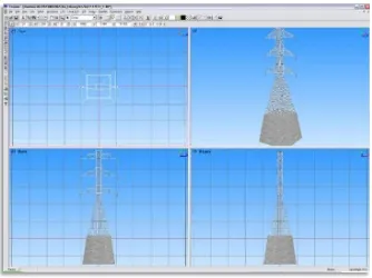
The goal of this guidance is to model a typical high voltage electrical pylon resembling the one in the following figure. This guideline is based on version 3.1 of the CDB Best Practice, but is applicable to version 3.0 as well1.

Figure 6-1: Typical Electrical Pylon

6.1.1 Pylon Model Orientation

The front (and back) of a powerline pylon is aligned with the general direction of the attached wires as illustrated below.

(10)

Figure 6-2: Pylon Orientation

The above snapshot is similar to the one found in Figure 6–10 of CDB Best Practice - Volume 6: OGC CDB Rules for Encoding Data using OpenFlight.

6.1.2 OpenFlight Graph

The OpenFlight graph of the above pylon exposes the 3 cross-arms, each with 2 insulators where wires are attached. Here are the names of the components that are used to model this power pylon:

• Pylon (global zone)

• Arm (horizontal cross-arm at the top of the structure)

• Insulator (ceramic insulator string attached at the end of each arm)

These 3 names are used to create CDB Zones as explained in section 6.5 of the CDB Best Practice: Volume 6 OGC CDB Rules for Encoding Data using OpenFlight. Here is the first level of the resulting graph.

Pylon

Object Arm[1] Arm[2] Arm[3]

(11)

Arm[n]

Object Insulator[1] Insulator[2]

Again, Object represents the steel structure of the cross-arm without the insulators. When looking at one of the cross-arm of the power pylon from the back, Insulator[1] is to the left while Insulator[2] is to the right. Finally, each insulator has an attach point to indicate where to connect an eventual wire.

Insulator[n]

Object Attach_Point

The node Object contains the geometry of the insulator.

As explained in section 6.8 of the CDB Best Practice Volume 6: OGC CDB Rules for Encoding Data using OpenFlight, the resulting list of paths is as follow:

• \Pylon

Note the presence of a total of 6 attach points (1 attach point per insulator × 2 insulators per cross-arm × 3 cross-arms per pylon = 6 attach points per pylon). Even though all attach points have the same name, there is a unique path to reach each one. For this reason, there is no ambiguity identifying and locating each point.

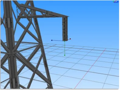
6.1.3 Attach Point Orientation

(12)

orientation of the Z-axis. Make sure to leave the Y-axis in the direction of the wire as in the figure below.

Figure 6-3: Attach Point Orientation

In this figure, the position and orientation of the attach point is identified by the blue-red -green axis system beneath the insulator. The Y-axis is in red and points in the same direction as the model’s Y-axis, which is toward the front of the model. The Z-axis is in green and points down indicating that wires attach under the insulator.

6.2 Guideline: Generating Wires between Pylons of a Powerline Formerly Annex A.2 in the CDB Best Practice, Volume 2.

This guideline is intended for both modelers and developers responsible for the creation of:

• CDB content such as 3D models representing pylons

• Tools used to generate the Powerline Network datasets

(13)

6.2.1 Powerline Network Attributes

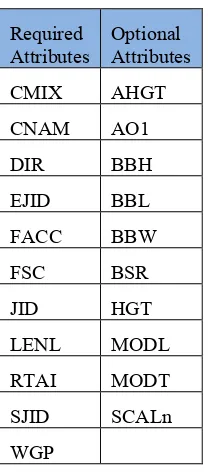
As a result of the above tables, a CDB-compliant Powerline Network dataset requires 11 mandatory attributes (listed in the first column of Table 6-1). Optionally, when a 3D model representing a pylon is provided, 4 additional attributes are required (MODL

2

(14)

obviously, plus BSR, HGT, and MODT) and 5 others remain optional (AO1, BBH, BBL, BBW, and SCALn).

6.2.2 Generation of HGT

The HGT attribute represents a special case because table 5-47 suggests that the attribute is optional while, in fact, it should always be present. If you carefully read its description in paragraph 5.3.1.2.3.17, you realize that HGT is required in both the line and figure point features of the Powerline Network.

For line features, HGT represents the average height above ground of the powerline when no MODL is specified, as suggested by the discussion about HGT in section 5.3.1.17 of the CDB Standard Volume 1: OGC CDB Core Standard: Model and Physical Data Store Structure In the figure point features, HGT represents the height above ground of the pylon, whether or not a MODL is provided. In either file, when MODL is supplied, HGT represents the height of the 3D model above the ground.

You should read guideline (6.3 – old Annex 6.3) for a complete discussion about HGT

6.2.3 Pylon Orientation

If the orientation of the pylon is specified by AO1, then use the value as-is. If the orientation is not specified, the client device must compute its value using the orientation of the segments of the line that are adjacent to the pylon. In the case of the first and last segments, the orientation of the segment is also the orientation of the pylon. For the other segments, the orientation of the pylon is the average of the orientation of the two adjacent segments.

6.2.4 Number of Wires

When no MODL is provided at all – meaning no MODL for the line and none for the figure points – and because there is no attribute specifying the number of wires along the transmission line, the client device must assume a generic powerline with two wires separated by a width of WGP meters connecting generic posts (simple pylons) of HGT meters high.

When a common MODL is specified for the whole line and no figure points are provided, it is possible to determine the number of wires by counting the number of attach points in the 3D model. Refer to guideline 6.1.2 (old 6.1.2) for details on how to detect attach points.

(15)

6.2.5 How to Connect Wires to Attach Points

If the client device has a single generic pylon along the line, then there is no problem connecting wires and attach points. That is when multiple pylons are used along the same line that problems arise. The client has to match attach points from one type of pylon to attach points on another pylon that may be of a different type. The algorithm to determine how to connect pylons of different types is left to the client device. A future version of CDB Standard will provide a robust and deterministic approach on how to connect the wires.

6.3 Guideline: How to Interpret the AHGT, HGT, BSR, BBH, and Z Attributes Formerly Annex A.3 in the OGC CDB Best Practice, Volume 2.

The goal of this guideline is to promote a correct use of five CDB attributes: AHGT, HGT, BSR, BBH, and Z. The article is aimed to both developers and users of content creation tools as well as developers of client applications.

A picture being worth a thousand words, the following diagram should help understand the relations between the AHGT, HGT, BSR, BBH, and Z attributes.

Here is a reminder of what these attributes are. The complete definitions can be found in Section 5.3.1.3, CDB Attributes in the CDB Standard Volume 1: OGC CDB Core Standard: Model and Physical Data Store Structure.

• AHGT (Absolute Height) is a flag to interpret correctly the value of the Z coordinate of a feature. When false, the value of Z is relative to the ground (Zr); when true, Z is the absolute altitude (Za).

• AHGT is not related with HGT even though their names are similar.

• HGT (Height Above Surface Level) is the distance from the top of the model to the ground.

• BBH (Bounding Box Height) is the distance from the top of the model to its XY plane.

• BSR (Bounding Sphere Radius) encompasses the portion of the model that is above its XY plane.

• Z is the altitude of a feature, either absolute or relative to the ground.

In the diagram above, a model (MODL) is positioned above the ground. This is indicated by the fact that the model’s XY plane does not lie directly on the ground. The distance

(16)

above the ground is represented by Zr. The diagram clearly shows the relation between HGT, BBH, and Zr.

�� ₌_��+_��

When the value of Zr is not readily available from the instance of the feature itself (because AHGT is true), it can be computed using the ground height (Gh).

�� =��₋�ℎ

The BBH attribute is optional and defaults to twice the value of BSR, which is mandatory for a MODL model.

��= 2×��

�� ≥��_��

6.3.1 Typical Use-case

Typically, a model is positioned relative to the ground without any offset. As a result, AHGT is false, and Zr is set to zero. Hence…

��₌ _��

6.3.2 Light Points

In the case of airport and environmental light points, no model of a light fixture is provided (the MODL attribute is not allowed). Hence…

��₌0 _→_�� ₌0

Currently, the light point datasets do not allow the HGT attribute, the client application may have to compute its value using the equation given previously…

�� ₌_��+_��

where BBH is null.

��₌ _��

And if the light point is positioned at an absolute height (AHGT is true), then…

�� ₌��₋�ℎ

6.3.3 Recommendation

Refrain from using AHGT. There are several advantages to leave this flag to false. First, it facilitates the creation of CDB datasets that are independent of each other. When the Z coordinate (altitude) of a feature is relative to the ground, the elevation dataset can be updated without the need to re-compute and update all features that have an absolute altitude.

(17)

the data store itself? No, this is not an error. It is perfectly possible to create content that is valid and – still – produce an incorrect result at the client level. Consider a feature that is positioned with an absolute height in a valley between two mountains of a high resolution terrain profile. At coarse LOD of terrain elevation, the valley and the mountains may (and will) be flattened producing a terrain skin that may no longer pass underneath the feature. Now imagine a client that uses that coarse LOD of elevation to create a terrain skin and then draw the feature at its absolute altitude, which happen to be underneath the terrain skin. The feature will not be visible or will be partially occluded by the terrain.

These reasons explain why the use of the AHGT flag should be avoided whenever possible.

6.3.4 When should AHGT be used?

Limit the use of AHGT to data whose source is inherently absolute. Such source data include geodetic marks or survey marks that provide a known position in terms of

latitude, longitude, and altitude. Good examples of such markers are boundary markers between countries.h

6.4 Guideline: How to Model a Wind Turbine

Formerly Annex A.4 in the OGC CDB Best Practice, Volume 2.

This text proposes a way to create a 3D model representing an articulated wind turbine. The articulations of interest are the yaw control to orient the turbine in the direction of the wind, the roll control to allow rotation of the rotor, and, optionally, the pitch control to change the orientation of the blades, if needed.

Beside is a typical Horizontal Axis Wind Turbine. The components of interest are the following:

The CDB metadata folder provides the proper code for a Wind Turbine, AD010-0053. The

(18)

code indicates the presence of a man-made point feature. individual control of the pitch of each blade is required, the Blades object (the lower right node) could be replaced with three (3) sub-trees each containing a Blade zone, a DOF node, and an object node.

With the proposed layout, a client device will detect the presence of a wind turbine through its feature attribute code (aka feature code), and recognize and control two articulations, the Turbine Yaw angle, and Rotor Roll angle.

A last note: to comply with the prescribed orientation of the CDB coordinate system as defined in section 6.3 Volume 6: OGC CDB Rules for Encoding Data using OpenFlight, the rotor must represent the front of the wind turbine (and not its right side).

Reference: http://en.wikipedia.org/wiki/Wind_turbine 6.5 Guideline: Handling of Model Interiors

CDB introduces the concept of the interior of a 3D model. The concept is developed in section 6.18, Model Interior, of the CDB Standard Volume 6: OGC CDB Rules for Encoding Data using OpenFlight. The following text serves as a complement to the standard to understand how the concept has been developed and how model interior is intended to be used.

6.5.1 Relationship between Model Shell and Model Interior

The ModelInteriorGeometry dataset is a subordinate dataset of the ‘regular’ ModelGeometry dataset. It depends directly on it. This is best illustrated by an example.

LOD ModelGeometry

6 Medium Shell Medium Interior

7 - -

8 Fine Shell Fine Interior

(19)

10 Finest Shell Finest Interior

11 - - ModelGeometry dataset. In this example, the model appears at LOD 2, a better version exists at LOD 6, an even better at LOD 8, and finally, the most detailed shell is at LOD 10. The Interior column shows 3 different LODs of interiors. There cannot be more Interior LODs than Shell LODs. Also, once an interior is provided (here at LOD 6), it must be provided for all subsequent (finer) LODs of the shell (LOD 8 and 10). Which means… interior at LOD 8 and 10 must exist.

6.5.2 Detecting Presence of a Model Interior

It is expected that a client will first request the shell of the model, then discover that the model has an interior because of the presence of a CDB Zone whose name is Interior (see 6.18.2 Volume 6: OGC CDB Rules for Encoding Data using OpenFlight, Pseudo-Interior), and then decide if the pseudo interior is sufficient for the application or if the real interior is necessary.

6.5.3 Access of a Model Interior

Client applications that are interested in 3D models will typically perform the following sequence of actions:

1. Load the GS Features of a tile

2. Load the GS and GT Models referenced by the GS Features

3. For each model, traverse its graph and detect the presence of an optional Interior (Zone name = Interior)

4. Decide to load the corresponding Interior (or not)

Interior datasets exists for both geospecific and geotypical models; hence, all features can be represented by a 3D model and all 3D models can have a separately modeled interior. Note the symmetry between the file names of shell and interior datasets. For geospecific models, the names of geometry files are…

• GeoCell_D300_{_S001_T001_Lxx_Ux_Rx_FeatureCode_FSC_MODL.flt}

• GeoCell_D305_{_S001_T001_Lxx_Ux_Rx_FeatureCode_FSC_MODL.flt}

For geotypical models, the file names become…

• D510_{_S001_T001_Lxx_FeatureCode_FSC_MODL.flt}

• D515_{_S001_T001_Lxx_FeatureCode_FSC_MODL.flt}

(20)

6.5.4 UHRB vs CDB Object Models

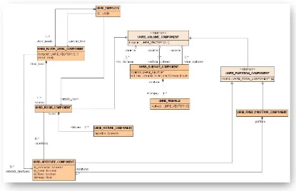
To help understand how CDB Model Interior maps to UHRB concepts, three (3) diagrams are provided below. The first two diagrams illustrate the UHRB Object Model4 while the third diagram presents the corresponding CDB Object Model.

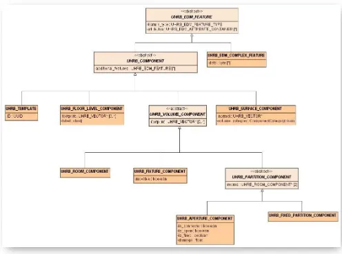
The first diagram is the UHRB Class Diagram presented in Figure 6-4 below. The class

diagram presents twelve classes of which eight are concrete classes that can be used to represent tangible objects. The UHRB_EDM_COMPLEX_FEATURE class implements an extension mechanism that is not required in the context of the CDB Specification. The remaining seven UHRB classes will be mapped to CDB zones.

Figure 6-4: UHRB Class Diagram

The second diagram is the UHRB Association Diagram of Figure 6-5; it shows all permissible associations between the UHRB classes.

(21)

Figure 6-5: UHRB Association Diagram

(22)

Interior

Figure 6-6: CDB Model Interior Object Model

6.6 Guideline: Applying Constraints to Uniformly Gridded Terrain Formerly Annex A.6 in the OGC CDB Best Practice, Volume 2.

(23)

Note that the rendering outcome into the Elevation dataset may vary depending on the rendering order of overlapping points, lines or polygons (polygons). In order to achieve deterministic outcome by all types of client-devices, client-devices are required to sort features by their layer priority number LPN before using them to constrain the terrain elevation dataset.

The rendering of a point, a linear or polygon (polygon) features into the Uniformly Sampled Terrain Elevation dataset is performed into the same LOD as the LOD in which the vector feature appeared.

6.6.1 Constraint Points

This section describes the required client-device behavior for PointZ and MultiPointZ features used as terrain elevation constraint points (AHGT is true) into a uniformly sampled terrain elevation dataset.

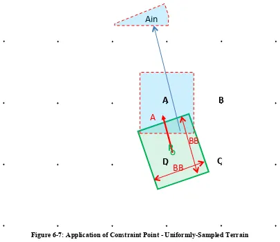
The application of a constraint point P is very much like drawing an anti-aliased rectangle centered on P into the uniform terrain elevation grid. The rectangle shape is defined by feature attributes BBL, BBH and AO1. Consider a terrain grid element A in the immediate vicinity of a constraint point P. After applying the constraint P to terrain grid element A, the new elevation �_!is:

�! = �! ∗��!"+ �!∗ ��!"

where…

�! is elevation of grid element A

�! is elevation of constraint point P

��

!" is the percentage overlap of constraint point P onto grid

element A

��

(24)

Figure 6-7: Application of Constraint Point - Uniformly-Sampled Terrain 6.6.2 Constraint Linear Features

This section describes the required client-device behavior for PolyLineZ features used as terrain elevation constraint linear feature (AHGT is true) into a uniformly sampled terrain elevation dataset.

First, the PolyLineZ feature is broken into a series of constraint lines. The application of each constraint line L is very much like drawing an anti-aliased line centered on L into the uniform terrain elevation grid. The width of the line is defined by feature attribute WGP. Consider a terrain grid element A in the immediate vicinity of a constraint line L, defined by vertices V1 and V2. After applying the constraint line L to terrain grid element A, the new elevation �_!is:

�! = �!"∗��!"+ �!∗ ��!"

where…

�_! is elevation of grid element A

�_!" is interpolated elevation of constraint line L at grid element A

A

_B

C

D

Ain

A

(25)

��

!" is the percentage overlap of constraint line L onto grid

element A

��

!" = 1 − ��!"

Figure 6-8: Application of Constraint Line - Uniformly-Sampled Terrain 6.6.3 Constraint Polygons

This section describes the required client-device behavior of PolygonZ and MultiPatch features used as terrain elevation constraint points (AHGT is true) into a uniformly sampled terrain elevation dataset.

Each vector PolygonZ feature consists of a number of rings (or parts). Each ring is a closed (the first vertex is same as the last vertex), non-self-intersecting loop. A PolygonZ feature may contain multiple outer rings. A sequence of rings can describe a convex or concave feature outline. In the CDB standard, rings can only be made up of triangles.

V

A

V

Ai

n

(26)

Each vector MultiPatch feature consists of a number of rings (or parts). Each ring is a closed (the first vertex is same as the last vertex), non-self-intersecting loop. A sequence of rings can describe a convex or concave feature outline. While the vector MultiPatch feature permits multiple inner rings (aka parts), this capability is dis-allowed in CDB. Furthermore, rings can only be made up of triangles.

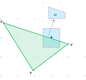
The rendering of the vector feature is handled as a series of constraint triangles applied in the order in which they appear within the vector PolygonZ record. The application of each constraint triangle T is very much like drawing an anti-aliased triangle into the uniform terrain elevation grid. Consider a terrain grid element A in the immediate vicinity of a constraint triangle T, defined by vertices V1, V2 and V3. After applying the constraint triangle T to terrain grid element A, the new elevation �!is:

�! = �!" ∗��!" + �! ∗ ��!"

where…

�! is elevation of grid element A

�!" is interpolated elevation of constraint triangle T at grid element A

��

!" is the percentage overlap of constraint line T onto grid

element A

��

(27)

Figure A-9: Constraint Polygons

6.7 Guideline: Applying Constraints to Non-Uniform Gridded Terrain (A.7)

The following sub-sections describe the rendering of point, line and polygon (polygons) into a Non-Uniformly Gridded Terrain Elevation dataset described in addendum “CDB Standard Addendum – Non-Uniform Sampled Terrain Elevation”

Note that the rendering outcome into the Elevation dataset may vary depending on the rendering order of overlapping points, lines or polygons. The Layer Priority Number (LPN) attribute is used to achieve deterministic outcome by all types of client-devices. When ECP is supplied, client-devices are required to sort overlapping constraint points, lines and polygons in low-to-high order and then render them in that order. Value of LPN can range from 0-32767.

The rendering of a point, a line or polygon features into the Non-uniformly Sampled Terrain Elevation dataset is performed into the same LOD as the LOD in which the vector feature appeared.

V

A

V

Ai

(28)

6.7.1 Constraint Points

This section describes the required client-device behavior for PointZ and MultiPointZ features used as terrain elevation constraint points (AHGT is true) into a non-uniformly sampled terrain elevation dataset.

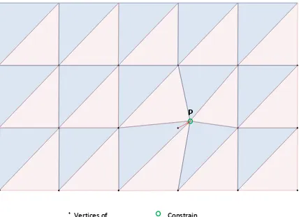
The application of a constraint point P is applied as follows:

1. The x,y address of the affected terrain grid element is computed by truncating the lat-long coordinates of point P; note that the truncation operation varies in accordance to LOD of the terrain; however, it always yields grid element addresses in the range of 0-1023.

2. The x,y offset of the affected terrain grid element is computed by performing a MOD of the lat-long coordinates of point P in accordance to its LOD.

Figure 6-9: Application of Constraint Point – Non-uniform Grid 6.7.2 Constraint Linear Features

This section describes the required client-device behavior for PolyLineZ features used as terrain elevation constraint line (AHGT is true) into a non-uniformly sampled terrain elevation dataset.

Vertices of Constrain

P

(29)

First, the PolyLineZ feature consisting of n vertices is broken-down into (n-1) line segments defined by successive pairs of vertices.

The application of a constraint line segment L is applied as follows:

1. The x,y offsets of the grid elements of each vertex are computed. (see application of constraint points into non-uniformly sampled terrain (case 1).

(30)

Figure 6-10: Application of Constraint Line – Non-uniform Grid 6.7.3 Constraint Polygons

This section describes the required client-device behavior of PolygonZ and MultiPatch features used as terrain elevation constraint points (AHGT is true) into a non-uniformly sampled terrain elevation dataset.

Each vector PolygonZ feature consists of a number of rings (or parts). Each ring is a closed (the first vertex is same as the last vertex), non-self-intersecting loop. A PolygonZ feature may contain multiple outer rings. A sequence of rings can describe a convex or concave feature outline. In the CDB standard, rings can only be made up of triangles. Each vector MultiPatch feature consists of a number

of rings (or parts). Each ring is a closed (the first vertex is same as the last vertex), non-self-intersecting loop. A sequence of rings can describe a convex or concave feature outline. While the vector MultiPatch feature permits multiple inner rings (aka

Vertices of Constrain Line Constrain Line

V

(31)

parts), this capability is dis-allowed in CDB. Furthermore, rings can only be made up of triangles.

The application of a constraint triangle T is applied as follows: 1. The x,y offsets of the grid elements of each

vertex are computed. (see application of constraint points into non-uniformly sampled terrain (case 1).

2. The x,y offsets of all the other grid elements that are intersected by the line segments are handled in accordance to the illustration shown here. (case 2 to Case 5)

(32)

Figure 6-11: Application of Constraint Polygon – Non-uniform Grid

6.8 Guideline: LOD Read Behavior of Subordinate Datasets (A.8)

In the CDB Standard, LOD read behavior of subordinated datasets was mentioned only briefly in…

• Section 5.2.1.2.3 Subordinate Terrain Elevation Components (Volume 1: OGC CDB Core Standard: Model and Physical Database Structure) which stated “The CDB standard does not permit the use of subordinate Terrain Elevation component when the primary Terrain Elevation component is not generated.” • Section 5.2.1.3.4 Default Read Value: which stated “Simulator client-devices

should assume … if the data values are not available (files associated with the Subordinate Terrain Elevation component for the area covered by a tile, at a given LOD or coarser, are either missing or cannot be accessed).

• Section 5.2.1.6 Subordinate Bathymetry Component: which stated “Furthermore, since the Bathymetry values are relative to Terrain Elevation component, each value in the Bathymetry component must be matched to the finest available LOD elevation values of the Terrain Elevation component”.

Vertices of Constrain Triangle Constrain Triangle

V

(33)

• Section 5.2.1.7.3 Default Read Value: which stated “Simulator client-devices should assume … if the data values are not available (files associated with the Subordinate Terrain Elevation component for the area covered by a tile, at a given LOD or coarser, are either missing or cannot be accessed).

• Section 5.2.2.3.2 Default Read Value: which stated “Simulator client-devices should assume … if the data values are not available (files associated with the Subordinate Terrain Elevation component for the area covered by a tile, at a given LOD or coarser, are either missing or cannot be accessed).

This guideline provides clarification on the client-device LOD read behavior of subordinated datasets; it describes the mandated behavior of a simulator client-device when reading a LOD of a Primary Elevation Component and combining it with another LOD of a Subordinate Terrain Elevation Component

Consider the case where a simulator client-device is attempting to read CDB data for a given region of the CDB at LOD = p. The CDB region has a Primary Elevation Component populated with data ranging from LOD = -10 to LOD = m, and a Subordinate Elevation Component populated with data ranging from LOD = -10 to LOD = n.

The required client-device read behavior is illustrated in Figure 6-12 below, and can be

• For -10 ≤ p ≤ n, the client-device accesses the subordinate elevation data at LOD = p.

• For p > n ≥ -10, the client-device accesses the primary elevation data at LOD = n.

• For p > m and p < n and m < n, the client-device interpolates the primary elevation data from LOD = m to LOD = p before combining it with the subordinate elevation data of LOD = p.

• For p > m and p > n and m < n, the client-device interpolates the primary elevation data from LOD = m to LOD = n before combining it with the subordinate elevation data of LOD = n.

• For p < m and p > n and m > n, the client-device interpolates the subordinate elevation data from LOD = n to LOD = p before combining it with the primary elevation data of LOD = p.

(34)

• For n = φ (unavailable) and p > m ≥ -10, the client-device accesses the default value in Defaults.xml for the subordinate elevation data.

• The combination of (m = φ (unavailable) and n ≥ -10), is not permitted, i.e., the generation of Subordinate Terrain Elevation LODs is not permitted if the Primary Terrain Elevation component have not been generated.

• If the default value for the Primary Elevation dataset is unavailable in Defaults.xml, or if Defaults.xml file is missing, then the client-device must revert to the client-device’s internal default value for this dataset.

• If the default value for the Subordinate Elevation dataset is unavailable in Defaults.xml, or if Defaults.xml file is missing, then the client-device must revert to the client-device’s internal default value for this dataset.

Figure 6-12: Client-device Read Behavior

(35)

The default values for the Subordinate Terrain Elevation layer “n” (where “n” is the subordinate elevation layer number, e.g., a value from 2 to 99) is the constant Subordinate_Elevation-n, which can be found in \CDB\Metadata\Defaults.xml. The CDB standard recommends that the value for Subordinate_Elevation-n = 0. In the case where the default value cannot be found within the Defaults.xml file, or that the Defaults.xml file cannot be found, the CDB standard recommends that client-devices internally generate a default value of Subordinate_Elevation-n = 0.

The CDB standard does not permit the use of Subordinate Terrain Elevation components when the Primary Terrain Elevation component is not generated.

6.9 Information: Tide Simulation Modeling Alternatives (Was A15) Formerly Annex A.15 in the OGC CDB Best Practice, Volume 2.

(36)

Figure 6-13: Examples of Ocean Tide Simulation Fidelity in Simulator

6.10 CDB and FalconView (Was A.16)

While the CDB file naming convention and its directory structure are somewhat different from that used in FalconView5, it is possible to find equivalent files between the two. The FalconView directory structure contains some metadata describing its content and area coverage; it has a three level directory structure. The first level “rpf” is a raster product format: the second level being the dataset such as “gnc” (global navigation chart): and the third level relates to the zones; all files are under the third level. The file name is eight characters long followed by a three-character file extension, and the file name portion uses a radix 34 numbering notation that is based on the position of the frame in the zone as well as revision info and the producer ID key. The file extension is based on the dataset and the zone. Note that frames are equivalent to CDB tiles.

From information such as a given lat/lon, a given resolution such as one-meter pixel size and the dataset such as global navigation chart, it is possible to generate the corresponding FalconView file name and its path. Similarly, given a lat/lon, an LOD and a dataset it is possible to generate a CDB file name and its path. Though not identical in coverage and resolution these two files should be similar in content for the same dataset.

5

(37)

Note that when given a CDB file name, it is possible to extract the tile position in lat/lon, the dataset it belongs to, and the LOD, even its full path name, i.e. the file name is unique for the entire CDB. This is not the case for FalconView. Since the resolution is not implicit in the name, the file itself must be read to extract this information; the dataset and zone info can be extracted from the file extension. Also note that directories in FalconView can potentially be very large since all files in a zone reside in the same directory; this is especially true for fine resolutions.

The FalconView directory structure follows the guidelines and conventions specified by MIL-STD-2411.

The algorithms used to find file name are given by examples within the MIL-C-89041 Controlled Image Base (CIB) document; in that document, zones are shown as overlapping. Note that this may not reflect the manner in which FalconView was implemented; nonetheless this does not affect the methodology provided in this section. 6.10.1 FalconView Directory structure

In FalconView, a top-level directory contains files that are metadata containing information about the various datasets and files in the directories.

The FalconView directory structure is as follows: Falconviewmaps

+---covdata Coverage data

| cgnc.cov Global Navigation charts | cjga.cov Joint Operation Graphics Air | cjnc.cov Jet Navigation Chart

| trs_8km.cov Township Range Section |

+---rpf Raster Product Format

| +---cgnc Global Navigation Map

| | +---1 Zone

(38)

6.10.2 FalconView Zones definition

MIL-STD-2411 divides the world into 18 zones, nine in the northern hemisphere and nine in the southern hemisphere. The first eight zones in both hemispheres are divided into frames, which in turn are divided into sub-frames. Frames are made of pixels with 1536 x 1536 pixels in a frame; there are 36, 6x6 sub-frames per frame. Between each zone, there is an overlap of one frame; this implies that the size of zones will vary slightly depending on the resolution that is used. T a b le 6 - 3 Z o n e s R a n g e N o O v e r l a p gives the

Along lines of constant longitude, the pixel constant used to determine the size of frames is a function of the resolution but is independent of the zone. Along lines of constant latitude the constant is a function of both resolution and zone and is based on the mid latitude of the zone. T a b l e 6 - 4 E x a m p le R e s o lu t io n e a s t - w e s t p ix e l c o n s t a n t s that is

extracted from MIL-C-89041 enumerates the factors for three resolutions.

T a b le 6 - 4 E x a m p l e R e s o lu t io n e a s t - w e s t p ix e l c o n s t a n t s

1,A 3,696,640 7,393,280 36,966,400

(39)

The north-south or latitudinal pixel constant is the number of pixels from the equator to the pole (90°). The east-west pixel constant is the number of pixels longitudinally from the 180° west longitude meridian going 360° in an easterly direction along the zone midpoint.

6.10.4 FalconView Zone extension based on resolution

To illustrate, we will use as an example a resolution of 10 meters. To calculate the exact latitudinal zone extent for a given resolution, first calculate the number of pixels in a degree of latitude for the resolution 11121.7777

90 integer. For example in the first zone the number of frames is 232

1536

In order to find the extent of the next zone we use the following method, which applies to all zones from 2 to 8 or B to H.

3,C 2,457,600 4,915,200 24,576,000

4,D 1,991,680 3,983,360 19,916,800

5,E 1,633,280 3,266,560 16,332,800

6,F 1,372,160 2,744,320 13,721,600

7,G 1,100,800 2,201,600 11,008,000

8,H 824,320 1,648,640 8,243,200

(40)

The number of longitudinal frames and subframes is computed by determining the number of subframes to reach around the earth along a parallel at the zone midpoint. The east-west pixel constant is divided by 256 pixels to determine the number of subframes. The results are divided by 6 and rounded up to obtain the number of frame columns.

For example longitudinally in the first zone we get 14440 Source Image GSD of 10 Meters, shows the complete set for a resolution of 10 meters.

Table 6-5 Frame/Subframe Sizes for Source Image GSD of 10 Meters

(41)

Zone Number Subframes

MIL-C-89041 states that “the origin for counting nonpolar frame rows and columns is the southernmost latitude of the zone and 180° west longitude, with columns counted in an easterly direction from that origin, as opposed to frames and subframes where “the origin for the subframe and pixel numbering within frames and subframes shall be from the

(42)

(

)

MIL-C-89041 for Controlled Image Base (CIB) states that:

“The naming convention for all resolutions of images registered in MIL-STD-2411-1, where it is intended for producers to provide contiguous [frame file] coverage, shall conform to MIL-STD-2411. In addition, the CIB [frame file] names are further restricted to conform to the form “ffffffvp.ccz.” The “ffffff” portion of the name shall be a radix 34 value that encodes the unique cumulative frame number within a zone in base 34, with the right-most digit being the least significant position. The radix 34 value incorporates the numbers 0 through 9 and letters A through Z exclusive of the letters “I” and “O” as they are easily confused with the numbers “1” and “0”. For example, the “ffffff” portion of the names would start with “000000,” proceed through “000009,” “00000Z,” “000010,” and so forth until “ZZZZZZ.” This allows 1,544,804,416 unique [frame file] names; a contiguous grid of frame names down to a resolution of 0.2 meters (approximately 8 inches) can be defined. The “v” portion of the name shall be a radix 34 value that encodes the successive version number. The “p” portion of the name shall be a radix 34 value that designates the producer code ID, as defined in MIL-STD-2411-1. The “cc” and “z” portions of the name extension shall encode the data series code and the zone, respectively, as defined in MIL-STD-2411-1. The CIB producers are responsible to ensure that [frame files] for all image resolutions, zones, and revisions, have unique names.”

In our case: _ffffff ₌F_C ₊F_R_×N_crz

… N z r

cztis thenumber ofcolumnsinzone for a resolution where

In the example of a lat of 36 and lon –88 with a resolution of 10 meters we get:

ffffff = 503+29x1970=57633 or 001FV3(34)

(43)

navigation chart dataset a version level 0, a manufacturer code of 3 and zone 2 the file name would be equal to “001FV303.GN2”

Note that nothing in the file name defines the resolution for the data; this information is part of the [coverage section] in the file itself (see section 3.12.3 in MIL-C-89041). Also note that the file name is unique only to the zone at a given resolution.

On the other hand a similar file for imagery (VSTI, Visible Spectrum Terrain Imagery) in the CDB convention for an LOD of 04 which has a resolution of approximately 8 meters; at position lat 36 and lon –88 we would get for the file name:

\CDB\Tiles\N36\W088\004_Imagery\L04\U0\ N36W088_D004_S001_T001_L04_U0_R0.jp2

Note that the file name itself is unique worldwide and that from it we can derive the directory path to which it belongs.

6.11 Managing CDB Data Store Versions (Was A.18)

The incremental versioning mechanism of a CDB data store provides a fast method of creating versions of the CDB data store changes since all the data changes are located under a single root directory. The creation and the managing of the (incremental) data files are however under the application control.

(44)

Figure 6-14: Concurrent Usage of CDB Versions

The underlying CDB versioning mechanism is a fine-grained file-level mechanism, i.e., only the affected files of the geographic areas of the CDB data store need to be versioned, leaving the rest of the CDB data store intact. This approach is invaluable in mission rehearsal applications where the target areas of the CDB data store require frequent updates based on the latest intelligence data.

The approach can also be applied to the handling of classified secure data. In this case, a CDB version can be used to hold the portion of the CDB data store that contains the classified information. The incremental versioning mechanism would be used to segregate the classified portion of the CDB data store onto a separate storage medium. Since the classified portion of the CDB data store is embedded within the overall CDB structure, it is possible for the runtime publishers to instantly switch back and forth between the classified and non-classified versions of the data store.

6.12 Guideline: Handling of GS and T2D Models (Was A.19) Formerly Annex A.19 in the OGC CDB Best Practice, Volume 2.

6.12.1 GSModels

6.12.1.1 GSModel Levels-of-detail

The insertion of a 3DModel-LOD into the LOD hierarchy of the GSModel Dataset is solely dependent on its Location, its Significant Size and on its Storage Size.

(45)

Figure 6-15: Handling Tile-LOD Overflows in GSModel Dataset

(46)

ensures that the modeled content is accessible in chunks that are bounded; this improves the allocation and management of memory allocation in the client-devices.

NOTE: The Significant Size of a 3DModel-LOD determines where it is nominally inserted into the 3DModel LOD hierarchy. In this nominal case, each Tile-LOD of the 3DModel Dataset holds a group of 3DModels-LODs that have similar Significant Sizes. This enables the client-devices to determine the range at which the 3DModel-LOD can be optimally blended-in to the scene (so that the model falls within a specified angular error criterion).

The bounding criterion of 3DModel Tiles can lead to LOD migration, thus breaking the relationship between the Significant Size of a 3DModel-LOD and the nominal CDB 3DModel-LOD it belongs to. As a result, client-devices can no longer guarantee the range at which the 3DModel-LOD will be blended-in to the scene. In effect, each time the 3DModel-LOD is migrated by one LOD, the client-device will likely shorten the range at which it is blended into the scene by a factor of 2X, leading to potentially distracting artifacts. The severity of the artifacts is proportional to the amount of content that has migrated to finer LODs and to the number of LODs by which the content has moved.

While the CDB standard allows the migration of 3DModel-LODs to finer LODs when Tile-LODs overflows are encountered, it is understood that this may lead to rendering artifacts that might be considered unsatisfactory. Consequently, it is strongly recommended that tools (that generate the CDB hierarchy) be designed to optionally disallow the migration of 3DModel-LODs to finer LODs upon overflows, and instead flag the overflow condition and then abort. Upon such cases, modelers can then re-assess which 3DModels should be discarded or remodeled in order to simultaneously satisfy the CDB bounding criteria and the application requirements.

Each of the 3DModel-LODs is nominally configured as LODs. The exchange-LOD mechanism assumes that client-devices gradually substitute a coarser 3DModel-LOD located in a coarser 3DModel-LOD with a finer 3DModel-3DModel-LOD located in a finer Tile-LOD.

(47)

Figure 6-16: Compacting the GSModel Dataset

In order to reduce the depth of the LOD hierarchy, the GSModel Dataset is post-processed and subjected to a “compaction” process, starting from the finest LOD (e.g. LODmax) and progressing to the coarser levels. The compaction process takes finer

(48)

coarser LODs until the parent LOD is packed to capacity. This approach ensures that the modeled content is accessible in similarly-sized chunks of processing; this provides the means to improve internal parallelism and pipelining (i.e. improves client-device determinism)

The access and selection of 3DModel-LODs is done through the GSFeature Dataset. Each of the Tile-LODs of the GSFeature Dataset contains a list of Features; each Feature in turn points to a 3DModel-LOD at the appropriate LOD. In effect, the appearance of a Feature (along with its modeled representation) and the evolution of its modeled representation are entirely controlled by the GSFeature Dataset. As a result, the 3DModel-LODs of a 3DModel need not be located in consecutive LODs of GSModel Dataset hierarchy.

6.12.1.2 CDB LOD versus GSModel Significant Size

Section 6.8.3 of CDB Standard Volume 6: OGC CDB Rules for Encoding Data using OpenFlight provides a set of guidelines to establish the values for Significant Size SSc and SSLOD for GSModels.

Table 3 1: CDB LOD vs. Model Resolution shows the nominal position of a GSModel within the LOD hierarchy of the GSModel Dataset. Note all of the GSModel-LODs of a GSModel normally fall within a range of 8 levels-of-detail (i.e. the smallest tile size the GSModel can sit on). However, it is possible to extend this range by breaking up a GSModel-LOD into several OpenFlight files.

Here is a summary of the rules required by the CDB standard in order to ensure deterministic operation from client-devices:

1. Each feature may have multiple modeled representations at progressively coarser levels of detail. Each of the modeled representations is referred to as a GSModel-LOD. In absence of pre-modeled coarser LOD representations, the tools may automatically generate coarser modeled levels-of-detail.

2. A GSModel-LOD consists of a group of polygons that represent a feature at a specific level-of-detail; this group of polygons shares a unique Model Identifier derived from the Feature Attribute Code a Feature Sub-Code (FSC), a Model Name (MODL or MMDC), the GSModel-LOD’s Significant Size SS’LOD.

3. Each GSModel has a distinct Significant Size SS’ value based on its dimensions. In turn, each GSModel-LOD of a same GSModel has a distinct Significant Size value SS’_LOD based on its modeled accuracy. 4. Insertion of a GSModel-LOD into the GSModel Dataset hierarchy

proceeds as follows. Starting with LODmax (LODmax is a variable set by the

user that sets the maximum depth of the LOD hierarchy) and progressing to coarser LODs…

a. For each Tile-LOD, create a Model_List that is constructed from the GSModel-LODs that straddle the Tile-LOD.

(49)

then add it to the Tile-LOD. Only the coarser GSModel-LODs of this GSModel are available for future insertion into the GSModel LOD hierarchy.

ii. If the GSModel-LOD is the coarsest LOD of the GSModel and its Significant Size is in accordance to Table 3 1: CDB LOD vs. Model Resolution, then insert it at this LOD of the hierarchy. If the GSModel-LOD matches the Tile-LOD, remove it from the list for the processing of the coarser Tile-LOD.

b. If the Model_List is less than GSModelFileSize, no further processing is required.

NOTE: The Storage Size of (statically-positioned) MModels is assumed to be zero.

c. The Model_List of each Tile-LOD is sorted in decreasing order of Diff, where Diff is the difference between the Significant Size SS of the Model and the Significant Size as specified in Table 2.

d. If the size of the Model_List is greater than GSModelFileSize, then (starting with the first entry in the sorted Model_List), Models are simplified one-by-one until the size of the Model_List is less than

GSModelFileSize. When a simplification occurs, the Model_List is

re-sorted using the Diff value.

e. If a) the Model_List is deemed non-reducible and b) the Model_List is still greater than GSModelFileSize …

i. If LOD <_LOD

max, then…

(1) a Temp_Model_List is created and initialized with the contents of the Model_list. Starting from the end of the Model_List, Models are removed one-by-one from the Model_list (starting with the first Model in the Model_List) and are copied into the Temp_Model_List until the Model_List reaches

GSModelFileSize.

(2) The Temp_Model_List is merged to the children Tile-LODs and the children are re-processed using steps 4a to 4e. The process is iterative, i.e., the “overflow” is propagated into the finer LODs of the GSModel hierarchy.

ii. Else…

(1) Models are removed one-by-one, starting with the first Model in the Model_List, until the Model_List is less than

GSModelFileSize. The corresponding GSModels are removed

(50)

NOTE: It is strongly recommended that GSModels be modeled using several GSModel-LODs, spanning a wide range of fidelity. The availability of many LODs ensures suitability of the resulting CDB for real-time use with a minimum degradation in fidelity. Conversely, a low number of LODs can lead to unacceptably large steps in fidelity.

NOTE: It is strongly recommended that the coarsest modeled LOD of GSModels have no more than 128 vertices; this reduces the likelihood that the coarsest modeled LOD need be propagated to a finer LOD of the hierarchy.

NOTE: This algorithm preserves the highest available modeled content while ensuring that the runtime constraint file size limits are respected. While the CDB data model allows for infinitely-sized GSModel-LODs, a client-device may refuse to render the GSModel-LOD if it has insufficient memory to load all of the OpenFlight files that make-up the GSModel-LODs.

5. Each GSModel-LOD is subject to an OpenFlight file size limit of

GSModelFileSize, i.e. several OpenFlight files, each within the

GSModelFileSize limit, can be used to represent a very complex

GSModel-LOD. Each of OpenFlight files that form the GSModel-LOD share the same GSModel-LOD Identifier (see rule 2) and GSModel-LOD origin. Client-devices must render the GSModel-LOD in its entirety, even if it is allocated to several OpenFlight files.

NOTE: While the CDB data model allows for infinitely-sized GSModel-LODs, a client-device may refuse to render the GSModel-LOD if it has insufficient memory to load all of the OpenFlight files that make-up the GSModel-LODs.

6. Each Tile-LOD is subject to a file size limit of GSModelFileSize.

7. All of the GSModel-LODs in a GSModel OpenFlight file are nominally exchange-LODs (see exception in next rule).

(51)

9. The finer modeled representation of a GSModel (i.e. a GSModel-LOD with a smaller Significant Size) always appears in finer LODs of the GSModel Dataset LOD hierarchy than a coarser GSModel-LOD.

10.A Tile-LOD cannot contain more than one GSModel-LOD of the same GSModel.

11.Once inserted into the GSModel Dataset LOD hierarchy, there is no mandatory requirement to clip the contents of a GSModel Tile-LOD against its Tile-LOD boundaries. However, the contents of the GSModel Tile-LOD cannot protrude Tile-LODs by more than ½_{the dimension of}

the Tile-LOD.

12.There is no mandatory requirement to have consecutive GSModel-LODs in consecutive LODs of Tile-LOD hierarchy; it is permissible to have gaps within the Tile-LOD hierarchy.

13.Gaps in the LOD file hierarchy of the GSFeature Dataset are not permitted. This may result in Tile-LODs that are empty (e.g. without any GSFeatures). The presence of an empty Tile-LOD file for the GSFeature Dataset indicates the availability of modeled content invoked by finer LODs of the GSFeature hierarchy.

6.12.1.3 Example – Insertion of a GSModel with 3 LODs into the CDB Hierarchy

Consider an industrial building 200m wide x 200m length x 10m high. The modeler has not supplied any values for its Significant Size, nor has he provided a value for RTAI. It is modeled in three distinct levels of detail as follows:

a) Coarsest level: 5 polygons b) Mid level: 60 polygons c) Finest level: 300 polygons

Based on this information, we can derive Significant Size values for each of the modeled representation as follows and determine where within the hierarchy each of the GSModel-LODs should be inserted:

a. Coarsest level-of-detail:

a. Compute the model’s Significant Size …

��₌ (coarsest LOD) of the model should be nominally inserted at LOD 3 of the Tile-LOD (assuming its file size limit is not exceeded)

b. Mid level-of-detail:

Volume 7: OGC CDB Data Model Guidance Formerly An A Volume Part 2DB-model-guidance

Open Geospatial Consortium

Volume 7: OGC CDB Data Model Guidance

Formerly Annex A Volume Part 2

Contents

i.

Abstract

ii.

Keywords

iii.

Preface

iv.

Submitting organizations

v.

Submitters

1.

Scope

2.

Conformance

3.

References

4.

Terms and Definitions

5.

Conventions

6.

Data Model Guidance

A

B

C

D

Ain

A

V

A

V

Ai

n

V

A

V

Ai

P

V

V

V

V

(

)

_B