MATRIX INCOME VARIETIES OF INDONESIAN LABOR FORCE AND ITS APPLICATION IN INDONESA | Canon | Journal of Indonesian Economy and Business 6254 67161 1 PB

(1)

Volume 27, Number 1, 2012, 44 – 72

MATRIX INDEX OF INCOME VARIETIES OF INDONESIAN LABOR

FORCE AND ITS APPLICATION IN INDONESA

Syarwani Canon

1

State University of Gorontalo

(syarwanic@yahoo.co.id)

ABSTRACT

Matrix Index of Income Varieties (MIVP) is an index, which is developed from the

variety co efficiency and statistic

χ

2 so that it will produce output totally as shown by

Index of Williamson/Theil, as regionally as Index of Theil, sectorally as Index of Gini.

Besides, Matrix Index of Income Varieties (MIIV) is able to identify which individual/

sector/region influence the draw of income inequalities above or below the average. In

application, MIIV will produce a maximal outcome if it is combined with Labor Force

Productivity Index.

The outcome of MIIV/MIVP in Indonesia shows that the high-income inequalities in

Indonesia are influenced by the contribution of regional economy, regional labor force

contribution, the characteristic of regional economic sector, and regional potentials of

each province.

Keywords:

income distribution, total, region, sector, regional sector

INTRODUCTION

The

1

efficiency and effectiveness of

tween-region economic performance, has

be-come a very important issue in the study of

spatial economic development. One of the

crucial spatial economic developments is the

income inequalities in region and in inter

re-gion that root from the problem of rere-gional

heterogeneity. But in solving such problem,

often macro indicators that assume

homoge-nous regional condition are used.

The mentioned macro indicators are

repre-sentative to regional evaluation in general, as

they are of average concept and the spreading

aspect of social economy inside the region and

inter regions. Even in the formula of the

peo-ple’s income distribution indicators, it is

as-sumed that the spread o income inside a region

and inter regions is homogenous. The

1_{This paper has been awarded as the third runner up} winner of JIEB’s Best Paper Award 2011.

ity of income and people’s distribution of

in-come is always most likely to happen. Such

problem takes place because of the

heteroge-neity of geographical position, potentials, and

the level of productivity that take place in

every region (Dumairy, 1999; dan Nurzaman,

1997).

(2)

2012 Canon 45

1998; Friedmann 1986 in Rukmana 1995).

According to Hoover (1977) in general, the

urban society’s income per capita is higher

than non-urban society, and this will continue

this way until there is a serious handling. The

research outcome of Hoch (1972) says that in

United States the level of urban society’s

income per capita is influenced by the urban

condition. The level of urban society’s income

per capita in the northern and western regions

is higher than the southern region, but in the

period 1929 -1962, the difference slowly and

gradually became smaller.

The outcome of such thought and research

is in line with the concept of

Generative

Growth Theory

and

Competitive Growth

The-ory

(Budiharsono, 1988).

Generative Growth

Theory

states that upon the country’s steady

economic development, many economic

problems can be solved. In this case, some

regions indeed will grow faster than other

re-gions and if all rere-gions enjoy the same quality

of economic growth, the process of income

distribution will keep continuing. In other

words, the quality of the national economic

growth in the less developed/retarded regions

can be elevated. While

Competitive Growth

Theory

; is based on the assumption that the

national economic growth rate is determined

by exogenous force, and seemed as it were

divided in some regions. This situation takes

place when the national economic growth rate

is low, so the other regions will be victimized.

In some analysis to see the quality of

be-tween-region income spread, regional income

per capita variable is always used, because

such variable is relatively more easily obtained

than other variables like economic sector’s

income per capita. More obviously, a

discus-sion on the analysis instruments that are often

used to measure the quality of between-region

income distributions will be presented later.

Williamson’s Index (WI), which was

in-troduced by Jeffrey G. Williamson (1965), is

an analysis instrument with which the quality

of a total income distribution of the whole

regions can be seen. Williamson proposed Vw

(weighed index) and Vuw (outweighed index)

to measure the level of inequality of a

coun-try’s income per capita at a certain time. From

the calculation, which he has conducted in

many countries it can be seen that the

be-tween-region income inequality is inclined to

show trend of an upside-down U. At the early

development the degree of between-region

income inequality increased, then stabilized

and finally decreased again. In certain

coun-tries, the U form is not fully applicable and

there were certain special variants. The WI

value will also produce a different outcome if

the region division experiences change such as

upon the Regency or Province new division.

Such phenomena are visualized in figure 1.

According to Gore in Nurzaman (2002), the

condition of development will be divergent if

the city/regency division is like Figure 1A.

Nevertheless, if a province is divided into

more cities or regencies, the development will

become convergent as shown in Figure 1B. In

that figure, it is assumed that the labor

pro-ductivity is spread evenly in every region of

observation. This condition is certainly more

caused by the use of data that assumes that the

society’s income in every region is

homoge-nous. While the fact shows that the society

living in a region is classified into many

eco-nomic sectors, and in every sector, the level of

the labor productivity is very various

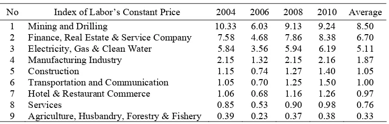
2

. At table

1, it is shown that Agricultural Sector,

Com-merce Sector, Hotel and Restaurant as well as

Service sectors are the three major sectors in

Indonesia wherein the lowest labor

productiv-ity level and the job opportunproductiv-ity are spread out

2_{The outcome of the observation by Canon (2008) in} calculating the level of labor productivity in each regional sector using Labor Productivity Index:

(3)

throughout all the regions. Besides, the three

sector at the average (from 2004-2010)

ab-sorbed 53,86 % of a total labor force, but only

produced a total output of 24,40% in

econ-omy.

On the other hand, the productive sectors

are influenced much by the natural resource

potentials and economic activity of the region

like technology, education quality, and

geo-graphical position all of which are not

spread/distributed evenly on the whole region

of observation. Certainly if regional division

takes place in a country or province, the

pro-ductive sectors will not be distributed evenly

throughout the whole regions, but will

possi-bly move to the region of division or will

re-main in the re-main region. This occurrence will

influence the change of William’s variant

In-dex value. That is why Nurzaman (2002)

states that it must be thought for what purpose

the Williamson Index analysis is carried out. If

the regional division is not appropriate for the

objectives of the study, it will give an absurd

analysis outcome and surely will bear

implica-tion on the deviated conclusion and the

target-missed policy. Mathematically, Williamson’s

Index value is derived from the coefficient

variety as found in the Equation 1.





N y y

n

i i



 

 1

2 2



(1)

A

B

Note:

Province Borders

City /Regency Borders

Source: Nurzaman (2002)

Figure 1.

The Inequality between Region and Different Regional Division

Table 1.

The Development of Indonesian Labor Productivity Index

No

Index of Labor’s Constant Price

2004

2006

2008

2010

Average

1 Mining

and

Drilling

10.33 6.03 9.13 9.24 8.50

2 Finance, Real Estate & Service Company

7.58

4.68

7.86

8.38

6.70

3 Electricity, Gas & Clean Water

5.84

3.56

5.94

6.19

5.11 4 Manufacturing

Industry

2.15 1.32 2.15 2.16 1.87

5 Construction

1.15 0.74 1.27 1.40 1.05

6 Transportation

and

Communication

1.05 0.70 1.25 1.50 1.00

7 Hotel & Restaurant Commerce

1.06

0.68

1.16

1.26

0.97 8 Services

0.85 0.53 0.90 0.98 0.76

9 Agriculture, Husbandry, Forestry & Fishery

0.39

0.23

0.37

0.38

0.33

(4)

2012 Canon 47

Value that results from coefficient variety in

the Equation 1 does not involve proportional

co- efficient in accordance with sub region,

and Williamson modified it so that it turns into

a weighed variant index as in the Equation 2.





y

p

y

WI

n

i

i i









1

2

(2)

Note :

y

i

= Regional income per capita to i

y

=

The whole regional income per

capita

p

i

= Regional population to i

p = The whole regional population

The other index model of income

inequalities that gives bigger attention to the

sub-regional aspect is Theil Index. This Index

was proposed by econometrician Henry Theil

(1967) from index entropy index. Entropy

index (Equation 4) has similarity to Wilks

Statistic or

l

ikelihood ratio that is stated in

Equation 3. But the research outcome of Zhao

et al.

(2006) shows that the level of type 1

error from heterogeneity test,

χ

2 statistic,

entropy statistic gives better result than

likelihood ratio statistic. In details, the

comparison among the heterogeneity test,

χ

2 statistic, entropy statistic, and likelihood

statistic has been experimented by Zhao

et al.

(2006) which is displayed at Figure 2. Based

on that figure, it is seen that

χ

2 statistic and

entropy statistic have similar pattern, while on

the contrary, likelihood statistic has different

pattern than the other two.





j ij

ij ij

E O O

G2 2 ln

(3)

Note:

O

ij

= Cell observation value

E

ij

= Cell expectation value

Based on the idea of entropy index, Theil

developed a measurement instrument to

cal-culate the inter-individual income inequality in

a group and the inter-group income inequality

(Equation 4).

F ig u re 1 : A s y m p to tic a v e ra g e v a lu e s fo r th e χ2, e n tro p y-b a se d , a n d lik e lih o o d -ra tio – b a se d h e te ro g e n e ity te s t sta tistic s a s a fu n c tio n o f th e fre q u e n c y p a ra m e te r f, u n d e r th e a ss u m p tio n s

n= 5 0 0 , f1=f, f2= 2f, f3= 3f, a n d f4= 1 -f1-f2-f3.

fig u re 2 : A s y m p to tic a v e ra g e v a lue s fo r th e χ2, e n tro p y-b a se d , a n d lik e lih o o d -ra tio – b a se d h e te ro g e n e ity te st sta tistic s a s a fu n c tio n o f th e fre q u e n c y p a ra m e te r f, u n d e r th e a ss u m p tio n s

n= 5 0 0 , f1= 4f, f2= 1 .5f, f3= 1 .5f, a n d f4= 1 -f1-f2-f3.

Source: Zhao et al. (2006)

(5)





Value at Equation 4 is divided into two

sections i.e. inequality between regions (

be-tween-region inequality

) and within region

inequality (

within-region inequality

) as shown

at Equation 5 and 6.

Theil’s Index has some strong points

compared to Williamson’s Index. This index

can calculate the income inequality between

sub regions within region, the income

ine-quality between regions, and the contribution

of each region/sub region towards the whole

income inequality. But Theil Index still uses

the same form of data as Williamson’s Index,

that is, income per capita. Income per capita

assumes that the quality of the society’s

in-come in every region/sub region of

observa-tion is homogenous. Such a problem can only

be overcome by Gini Coefficient, which was

developed by an Italian expert of statistic, i.e.

Gini (1912). Gini Coefficient is statistic

dispersion measurement towards the

dis-tribution of income group in a region. Gini

Coefficient value in several countries ranges

from 0,249 (in Japan) to 0,707 (in Namibia)

(Wikipedia, 2010). The data shows that the

quality of distribution of income of society

groups in every country on this world is

un-even. Based on that problem, it is necessary to

develop income distribution index that utilizes

sectoral and regional data. In the dimension of

regional size, such index can explain as much

as Williamson and Theil Index, while in the

dimension of sectoral size, it can explain as

much as Gini Index.

To arbitrate such problem, it is necessary

to develop a new index, so that it can explain

the income inequality either regionally or

sectorally. The new index is developed from

Williamson (Equation 2) that is combined with

χ

2 (Equation 5). In that index, variable



y_iy



with one measurement dimension is

replaced with



yijyeij



variable, which is a

variable with two-dimensional measurement.

In this case, the average value of population

income of sub region is replaced with

individ-ual value of expectation.

Value

y

ij

is value of income per capita of

region i sector j that replaces value y

i

as

re-gional income per capita. So does value

ij

ye

which is a value of expectation for each

individuals in equation that replaces the

aver-age value of

y

.

In Williamson Index every data, i.e.

in-come per capita of sub region is subtracted

with the income per capita of region



yiy



.

Whereas in the new index every data i.e.

in-come per capita of sub region is subtracted

with the value of ideal expectation



yij yeij



.

(6)

2012 Canon 49

To find out the value of income inequality

which comes above the average income

(posi-tive value) or below the average income

(negative value), it is necessary to simplify





in Equation 6 into





Equation 6 and Equation 7, which are two

similar equations, will bring about the same

value, but bring about different plus/minus

sign. The Equation 7 form will only bring

about the total value, whereas in finding the

total value in accordance with sector and

re-gion it is necessary to re-simplify Equation 8

(in accordance with region) and Equation 9 (in

accordance with sector).





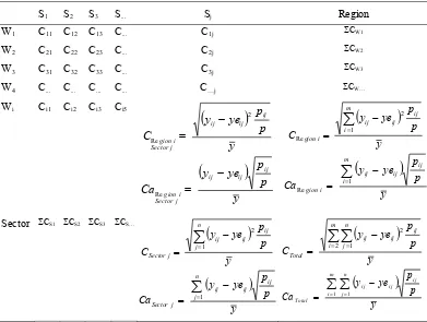
To find out value of every cell that shows

in-dividual of region i sector j, it is necessary to

re-simplify Equation 8 and Equation 9 into

Equation 10.

Equation 10 produces unique values as value

ICa in regional and sectoral sequence. Those

values are as negative values that range from

-1 to 0, or are as positive values that ranges

from 0 to 1. If the value reaches 0, the regional

sector will give lower influence toward the

region inequality, and on the contrary, if the

value reaches 1 or -1, the regional sector will

play bigger role in influencing the inequality

of regional income. Furthermore, if the index

value of regional sector is positive, the income

per capita of the regional sector is above the

average income per capita of the region

(y

ij

>ye

ij

). And in contrast to that, if the value

of regional sector’s index is negative, the

income per capita of regional sector is below

the average income per capita of the region

(y

ij

>ye

ij

). A further detail of description of

Matrix Index of Income Varieties (MIIV/

MIVP) is shown at Table 2.

(7)

Table 2.

The structure of Matrix Indoex of Income Varieties (MIIV/MIVP)

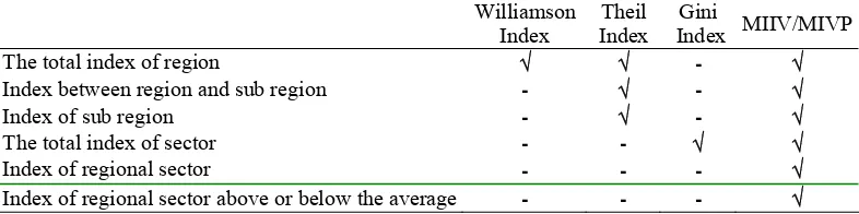
Subsequently, to make it more obvious in

seeing the difference among Williamson

Index, Theil Index, and MIIV/MIVP, a

simulation of the total of output value of the

three indexes. Whereas the data used in

calculating the three indexes is taken randomly

in fifty-time recurrence. Based on Figure 3, it

is seen that value MIIV/MIVP (the average

value C = 0,51 and Ca 7 = -0,02) is always

lower than Williamson Index value (the

average value IW=0,57). Thereafter,

Williamson Index value always produces

lower number than Theil Index (the average

IT=1,27)

3

. Based on Figure 3 it is also seen

that the movement pattern of curve of the three

indexes is quite alike, but MIIV/MIVP output

3_{In several references, it is explained that the value of} Williamson and Theil Index is between zero and one. But in several other studies like Nurzaman, the value of Williamson Index is bigger than one.

is more alike with Williamson Index. This

shows that although the average value of

Williamson (

y

) is replaced with expectation

value

 

yeij

as in MIIV/MIVP, both remain to

show almost the same output of performance.

Subsequently, value (C) at MIIV/MIVP

has the same interpretation as Williamson and

Theil Index, but Ca index at MIIV/MIVP has

different interpretation. If C value is combined

with Ca value, it will bring about a more

detailed description toward the causes of

inequality of income between regions. In more

detail, such explanation is shown at Table 3.

(8)

2012 Canon 51

-0,60 -0,40 -0,20 0,00 0,20 0,40 0,60 0,80 1,00 1,20 1,40 1,60

1 2 3 4 5 6 7 8 9 ₁₀ ₁₁ ₁₂ ₁₃ ₁₄ ₁₅ ₁₆ ₁₇ ₁₈ ₁₉ ₂₀ ₂₁ ₂₂ ₂₃ ₂₄ ₂₅ ₂₆ ₂₇ ₂₈ ₂₉ ₃₀ ₃₁ ₃₂ ₃₃ ₃₄ ₃₅ ₃₆ ₃₇ ₃₈ ₃₉ ₄₀ ₄₁ ₄₂ ₄₃ ₄₄ ₄₅ ₄₆ ₄₇ ₄₈ ₄₉ ₅₀

T

W

C

Ca

Note: W= Williamson Index, T= Theil Index, C=MIVP, Ca=MIVP +/- Source: Hypothetic Data.

Figure 3.

The Spread of Williamson Index, Theil Index, and MIIV/MIVP, Using Three-digit

Numbers in fifty-time Recurrence

Table 3.

The Comparison between C value, with Ca +, Ca-

Ca

C

Ca +

Ca -

Ca

≈

0 C

High

The high inequality caused

by certain regional sector

with the level of income per

capita above the average.

(experiment 36 and 37)

The high inequality caused

by certain regional sector

with the level of income per

capita below the average.

(experiment 29 and 46)

The high inequality, but

regional sector with

balanced high and low

income per capita.

(experiment 18 and 48)

C

Low

The low inequality but some

certain regional sectors are

with the level of income per

capita above the average.

(Experiment 24 and 26)

The low inequality but some

certain regional sectors are

with the level of income per

capita below the average.

(Experiment 1 and 7)

The low inequality and

regional sector with the

level of balanced hing and

low income per capita.

(Experiment 32 and 49)

Table 4.

The Comparison of Value between Williamson Index, Theil Index, Gini Index and

MIIV/MIVP

Williamson

Index

Theil

Index

Gini

Index

MIIV/MIVP

The total index of region



-



Index between region and sub region

-



-



Index of sub region

-



-



The total index of sector

- -



Index of regional sector

- -

- 

(9)

DATA

The data, which is used in this research, is

a secondary data from BPS in the form of

con-stant value of PDRB in the elementary year of

2000 and Labor Force. Those data are divided

into 9 sectors and 33 provinces throughout

Indonesia. While the period of years used are

four years i.e. 2004, 2006, 2008 and 2010.

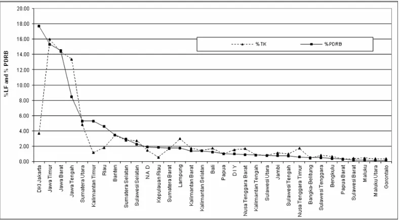
DISCUSSION

Economic Contribution (PDRB) and

La-bor Force (LF) from every province in

Indone-sia until very recently are not evenly spread

out. Figure 4, which uses the average data in

the year of 2004, 2006, 2008 and 2010, shows

that economic contribution and labor force

from several provinces across Indonesia can

be divided into four major groups, that is: (i) A

group, which consists of four provinces, i.e.

Jakarta until Central Java, with economic

contribution of 55.99% and LF of 47,43%. (ii)

A group, which consists of 6 provinces, that is,

North Sumatra province until South Sulawesi,

with economic contribution of 25,82% and LF

of 16,69%. (iii) A group that consists of 8

provinces, namely NAD province until Papua

with economic contribution of 12,26% and LF

of 12,53. (iv) A group that consists of 15

provinces, namely DIY province until

Goron-talo province with economic contribution of

7,93% and LF of 12,41%.

If looked carefully, the data description

for the four groups of provinces shows an

in-teresting condition, where there is a reversed

correlation between the amount of province

groups against the economic contribution and

the labor force given. A group of few

prov-inces gives a large economic contribution and

a very large number of labor forces. In

con-trast, a group of many provinces even only

gives small economic contribution and a small

number of labor forces. On the other side, it is

also seen that the quantity of labor forces (LF)

in each province is diametrically equal to the

quantity economic contribution (PDRB). The

explanation shows that in general, the

eco-nomic development in Indonesia is distributed

Source: calculated from BPS

(10)

2012 Canon 53

evenly and is still a compressed labor (

padat

karya

)

4

. These problems certainly require a

special attention considering that the major

economic generator in Indonesia still occurs

on the sector of Building Construction, and

Hotel and Restaurant Commerce, while the

sector of manufacturing industry is not

maxi-mally managed

5

. Despite the fact that

Indone-sia is famously rich of its primary sectors that

surely, require manufacturing industry to

pro-mote its added economic value. However,

be-cause of the minimum amount of

manufactur-ing industry of primary sector in Indonesia,

raw material that derives from this sector is

often used for export commodity. Of course,

this will bring about the lost opportunity for

the added economic value to elevate, and

budge to other countries. Besides, the

mini-mum number of manufacturing industry with

raw material of agricultural products will bring

about the impact of labor’s moving from

Agri-cultural sector to agriAgri-cultural-raw-material

based manufacturing industry sector. Whereas

in fact, in industrial Sector, the labor’s

pro-ductivity is much better than that in

agricul-tural sector. Therefore it is necessary to

de-velop economic analysis on the production

side to support the rapidly developed

eco-nomic analysis on the consumption side, so

that the national development program can run

more efficiently and effectively in line with

our expectation.

4

Canon (2007) research outcome in North Sulawesi Province (now, North Sulawesi and Gorontalo Pro-vince) shows that the population increase of this Province in short term has negative influence, but in long term has a positive influence towards the econo-mic development.

5_{Using sector analysis catalysis (Canon, 2010), the} sequence of sector catalysis group in Indonesia is as follows: 1) four other combined sectors include Hotel and Restaurant Commerce Sector, Building and Cons-truction Sector. 2) Two other combined sectors include Manufacturing Industry, Electricity, Gas and Clean Water Sector, Relation and Communication Sector, Rent and Service Finance Company, and Service Sec-tor. 3) other null combined sectors include Agricultural Sector, and Mining and Drilling Sector.

To make a matured and effective-efficient

planning, some analyses that can be used to

evaluate and to serve as the stepping basis for

making the future economic development

pro-gram are importantly required. One of the

analyses that can describe the labor’s income

varieties is the Matrix Index of Income

Vari-ety (MIIV/MIVP). MIIV/MIVP performs the

index of the labor’s income variety suited with

the province, sectors and province sector. The

outcome of MIIV/MIVP calculation combined

with the Labor’s Productivity Index (IPTK), is

quite interesting to bring up in this paper.

The development of labor force MIIV/

MIVP in provincial sequence in Indonesia for

the period of 2004, 2006, 2008 and 2010 is

quite various and very high. The total MIIV/

MIVP of Indonesia is as follows: year 2004 as

big as 1.53, year 2006 it dropped to 1.29, but

in year 2008 increased to 1.64 and in year

2010 dropped again to 1,23. It is estimated that

the increase of labor force’s variety index in

Indonesia in year 2008 resulted from the

global crisis that also hampered Indonesia.

Somehow the global crisis does not influence

the inequality of labor’s income in Indonesia

for a long time, because in 2010, the value

dropped again and even was lower than the

previous years. Then, from MIIV/MIVP

cal-culation in accordance with the province in

Indonesia, it can be concluded as the

follow-ing, that even though the value of variety

in-dex changes in that period, it does not change

the pattern of variety index value that takes

place.

(11)

East Kalimantan province give the largest

contribution toward the inequality of labor

force income in Indonesia. While provinces

that are relatively less influential to the

eleva-tion of the inequality of income in Indonesia

are West Sulawesi, Gorontalo and North

Maluku. As referred by Figure 4 and 5, it can

be seen that the amount of the positive variety

index in provincial sequence has correlation

with the amount of PDRB contribution

to-wards Indonesian economy. In other words,

the amount of the positive variety index that is

contributed by a province is diametrically

equal to the amount of percentage of PDRB

and Labor Force.

On the other side of Figure 6 it is

per-formed Positive Variety Index (IC),

Posi-tive/Negative Variety Index (ICa) and Labor’s

Productivity Index (IPTK) of the whole

prov-inces in Indonesia taken from the average

value in Year 2004, 2006, 2008 and 2010. The

figure shows that a pattern trend, in which the

smaller the IC value, the less ICa value will

fluctuate ,whereas the bigger the IC value, the

more the ICa value will fluctuate. Then, in

provinces with high IC and positive ICa, it

shows that high value of IC is caused by a

quite big draw of income above the average,

as what happens to Jakarta province, East

Kalimantan, Riau Province and several other

provinces. While provinces with high IC value

and negative ICa value show that the IC value

is caused by a quite big draw of income below

the average, as what occurs in Papua province,

Banten province, East Javanese province and

several others.

Subsequently, at figure 7 the average

sequence of province with highest ICa+ value

to the lowest value is made, and on the

contrary, province with the lowest ICa-value

to the highest one. Both combination of ICa+

and ICa – are ranked, then individually, are

correlated in the form of graphic line so that

they form an X letter.

(12)

(13)

That figure shows that most provinces with

high IPTK (Labor’s Productivity Index) in

Mining and Drilling Sector predominate the

right side position to letter ”X”, whereas

provinces with the highest IPTK (Labor’s

Productivity Index) in Rent and Service

Finance of Company predominate the left side

position to the cross of letter ”X”. This finding

shows that Mining and Drilling Sector gives

influence on the increase of income inequality,

on the other hand, Rent and Service Finance of

Company belongs to the group of sector

catalysis of Indonesia.

Figure 6 and Table 5 in general can

ex-plain that Jakarta province, East Kalimantan,

and Riau province are provinces with the

highest labor’s productivity and the largest

contribution toward the forming of the labor’s

income inequality in Indonesia. However,

when seen within the region itself like in

Ja-karta province and East Kalimantan, the big

income is mostly receieved by the middle

class society and above, while in Riau

prov-ince, the big income is received quite evenly.

As well as the other three provinces, Riau

province has the highest level of labor’s

pro-ductivity, but it only gives a small influence

toward the forming of income inequality in

Indonesia and the average income of the labor

force within its region is relatively distributed

evenly. In contrast with that, NAD province

region gives a medium influence toward the

labor’s income inequality and a productive

level of Labor’s productivity. North Sumatra,

Bangka Belitung, and Papua Barat provinces

are the region with productive labor force

(TK) with the contribution toward the

Indone-sian labor’s income inequality level from the

low to the very low level. Anyhow, when seen

from the condition of labor force within the

province itself, only North Sumatra province

that has Labor’s income level above the

average, whereas Bangka Belitung province

has a more evenly-distributed income.

Three groups of provinces that have

al-most productive labor force: The first group

consists of Papua, South Sumatra, Banten and

East Java province. The second group consists

of West Sumatra, West Java, West

Kaliman-tan, Central Java, Lampung province. The

third group comprises from South Kalimantan,

Central Kalimantan, North Sulawesi, South

Sulawesi, Central Sulawesi, Bali, Jambi, DIY,

and Southeast Sulawesi province.

The first province group gives medium

influence toward the forming of the level of

labor’s income inequality in Indonesia, and

within its region, many labors earn income

below the average. The second and the third

province group only gives a very small

influence toward the forming of income

inequality in Indonesia, besides within each

region of this province, the income of labor is

relatively even.

Last seven provinces which belong to the

less productive group, namely, Bengkulu,

NTB, West Sulawesi, Maluku, North Maluku,

Gorontalo, and NTT. It seems that this

prov-ince group also has two equivalent

occur-rences where their contribution toward the

forming of labor’s income inequality in

Indo-nesia is very low, and the level of labor’s

in-come in its province is relatively even.

(14)

2012 Canon 57

Table 5.

The Comparison among Positive Variety Index, Positive/Negative and Labor’s

Productivity Index in Provincial Sequence

No Wilayah IC ICa IPTK/LPI Explanation

1 DKI Jakarta, East Kalimantan

high above very productive

Contribution to the inequality of labor’s income in Indonesia is high with the labor’s income level above the average, with very high productivity level

2 Riau high evenly

distributed

very productive

Contribution to the inequality of labor’s income in Indonesia is high with labor’s income relatively even with high labor’s productivity.

3 N A D medium below productive Contribution to the inequality of labor’s income in Indonesia is medium, with labor’s income below the average, with high labor’s productivity.

4 Papua, South Sumatra, Banten, East Java

medium below almost productive

Contribution to the inequality of labor’s income in Indonesia is medium, with labor’s income within province below the average, with high labor’s productivity.

5 Riau Peninsula low evenly distributed

very productive

Contribution to the inequality of labor’s income in Indonesia is low, with labor’s income evenly distributed, with very high labor’s productivity.

6 North Sumatra low above productive Contribution to the inequality of labor’s income in Indonesia is low, with labor’s income within province evenly distributed, with high labor’s productivity.

7 Bangka-Belitung low evenly distributed

productive Contribution to the inequality of labor’s income in Indonesia is low, with labor’s income within province evenly distributed, with high labor’s productivity.

8 West Sumatra,

Contribution to the inequality of labor’s income in Indonesia is low, with labor’s income within province evenly distributed, with less labor’s productivity.

9 Papua Barat. very low

evenly distributed

productive Contribution to the inequality of labor’s income in Indonesia is very low, with labor’s income within province evenly distributed, with high labor’s productivity.

10 South Kalimantan,

Contribution to the inequality of labor’s income in Indonesia is very low, with labor’s income within province evenly distributed, with less labor’s productivity.

11 Bengkulu, NTB, West

Contribution to the inequality of labor’s income in Indonesia is very low, with labor’s income within province evenly distributed, with zero labor’s productivity.

(15)

0.000

Figure 8.

Positive Variety Index, Positive/Negative Variety Index and Labor’s Productivity in

Accordance with Average Sector, Year 2004, 2006, 2008, and 2010.

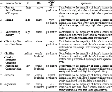
Table 6.

The Comparison among IC, ICa and IPTK/LPI (Labor’s Productivity Index) in

Accordance with Economic Sector.

No Economic Sector IC ICa IPTK/

Contribution to the inequality of labor’s income in Indonesia is high, with labor’s income within sectors above the average, with very high labor’s produc-tivity.

2 - Mining high below very

productive

Contribution to the inequality of labor’s income in Indonesia is high, with labor’s income within sectors below the average, with very high labor’s produc-tivity.

3 - Manufacturing Industry

high below productive Contribution to the inequality of labor’s income in Indonesia is high, with labor’s income within sectors below the average, with high labor’s productivity. 4 - Electricity, Gas

and Clean Water

medium above very

productive

Contribution to the inequality of labor’s income in Indonesia is medium, with labor’s income within sectors above the average, with very high labor’s pro-ductivity.

productive Contribution to the inequality of labor’s income in Indonesia is medium, with labor’s income within sectors evenly distributed, with high labor’s produc-tivity.

6 - Relation and Communication

low evenly distributed

productive Contribution to the inequality of labor’s income in Indonesia is low, with labor’s income within sectors evenly distributed, with high labor’s productivity.

7 - Services low evenly

distributed

almost productive

Contribution to the inequality of labor’s income in Indonesia is low, with labor’s income within sectors evenly distributed, with less labor’s productivity.

8 -Agriculture low evenly

distributed less productive

(16)

2012 Canon 59

Sector that holds the position of

produc-tive labor is: (i) Manufacturing Industry Sector

(ii) Building Sector, (iii) Hotel and Commerce

Sector, and (iv) Relation and Communication

Sector. The first sector gives the biggest

con-tribution to the forming of the inequality of

labor’s income, whereas the second sector

until the fourth sector gives a medium-to-low

contribution to the forming of the inequality of

labor’s income in Indonesia. While sectors

that belong to almost productive and less

pro-ductive, are; (i) Service Sector and

Agricul-tural Sector. Both sectors give the smallest

contribution to the forming of inequality of

income in Indonesia, besides the level of

la-bor’s income in both sectors is relatively

dis-tributed.

CONCLUSIONS

1. The amount of percentage of economic

contribution of the whole province in

In-donesia is diametrically comparable with

the percentage of labor force’s

contribu-tion. For Jakarta, Kalimantan, Riau, East

Kalimantan Province, the percentage of

la-bor is smaller than that of economy and the

three provinces give the biggest

contribu-tion to the total positive inequality index.

For Central Java, Lampung, NTB (West

Nusa Tenggara), and NTT (East Nusa

Tenggara), the percentage of labor is

bigger that of economy to the contribution

of the total positive inequality index. It is

low to the very low.

2. Based on the analysis outcome, basically, it

can also be concluded that the amount of

contribution to the total inequality index in

each province is influenced by the amount

of economic contribution of every

eco-nomic sector. The same thing is also

appli-cable where the amount of contribution of

the economic sector is diametrically

com-parable to the amount of contribution to the

positive inequality index.

3. The lower the contribution of a province to

the total inequality index, the more evenly

the level of labor’s income will be

distrib-uted within a province. On the contrary,

the bigger the contribution to the total

ine-quality indexes of a province, the more

various the level of the labor’s income

within a province will be.

4. The more productive the condition of labor

force within a province, the bigger

contri-bution the province will give to the total

income inequality index.

5. Sectors that play the most role in forming

the inequality of income in Indonesia is

sector of mining and drilling, and industry,

while sectors that play less role in forming

the inequality of income are sector of

agriculture and service.

6. In provinces with relatively high labor’s

income index (IPTK) on mining and

drilling sector will give impact on the

ele-vation of the level of income inequality

within its region. In contrast to that,

prov-inces with relatively high labor’s income

index on Rent and Service Finance of

Company will give impact on the decrease

of income inequality within its region.

REFERENCES

Budiharsono, S., 1989.

Perencanaan

Pemba-ngunan Wilayah (Teori Model

Perenca-naan dan Penerapannya)

[Regional

Development Planning (Theory,

Deve-loping Model, and its Application)].

Bogor: IPB.

Canon, S., 2010. “

Identifikasi Sektor

Katalisator dalam Perekonomian Wilayah

Provinsi Sulawesi Utara

[Identification of

Catalyst Sector in the economies of North

Sulawesi Province]”.

Jurnal Ekonomi dan

Pembangunan Indonesia

, 10 (2).

Dumairy, 1999.

Perekonomian Indonesia

[Indonesian Economy]. Jakarta: Erlangga.

Esteban, J., 1999.

Regional Convergence in

(17)

Hoch, I., 1972. “Income and City Size”.

Urban Studies

, 9, 299-329.

Hoover, E. M., 1977.

Pengantar Ekonomi

Regional [Regional Economies Preface]

.

Jakarta: LPFE Universitas Indonesia.

Nurzaman, S.S., 1997. “

Tinjauan Kesenjangan

Wilayah di Indonesia

[Regional

Discre-pancy Review in Indonesia]”.

Jurnal

Perencanaan Pengembangan Wilayah dan

Kota

, 8 (4).

Nurzaman, S.S., 2002.

Perencanaan Wilayah

di Indonesia (Pada Masa Sekitar krisis)

[Regional Planning in Indonesia around

the Crisis]. Bandung: Penerbit ITB.

Rukmana, D., 1995. “

Partisipasi Masyarakat

Dalam Kebijaksanaan Pengembangan

Wilayah Terbelakang

[Society’s

Partici-pation in Policy of Development in

Underdeveloped Region].

Jurnal

Perenca-naan Pengembangan Wilayah dan Kota

,

19. Theil, H., 1967. Economics and Information

Theory. Amsterdam: North Holland.

Wikipedia, “Gini Coefficient”, available at

http://en.wikipedia.org/wiki/Gini_coeffici

ent, accessed at June 27, 2010.

Williamson, J. G., 1965. “Regional Inequality

and the Process of National Development:

a Descryiption of the Patterns”.

Economic

Development and Cutural Change,

XIII

(4), 3-84.

Zhao J., E. Boerwinkle, and M. Xiong, 2006.

(18)

2012 Canon 61

APPENDICES:

Index C

2010 I II III IV V VI VII VIII IX Region

1 N A D 0.005 0.055 0.037 0.011 0.011 0.003 0.004 0.031 0.013 0.077 2 North Sumatra 0.018 0.071 0.027 0.010 0.006 0.008 0.021 0.050 0.010 0.096 3 West Sumatra 0.012 0.059 0.010 0.012 0.000 0.005 0.044 0.000 0.029 0.082 4 Riau 0.049 0.628 0.096 0.067 0.074 0.095 0.088 0.173 0.067 0.684 5 Jambi 0.004 0.001 0.005 0.004 0.009 0.005 0.008 0.004 0.008 0.018 6 South Sumatra 0.066 0.188 0.052 0.026 0.014 0.050 0.058 0.049 0.035 0.230 7 Bengkulu 0.008 0.010 0.017 0.000 0.005 0.007 0.007 0.009 0.012 0.028 8 Lampung 0.015 0.095 0.036 0.001 0.011 0.007 0.003 0.073 0.002 0.127 9 Bangka-Belitung 0.022 0.072 0.017 0.001 0.009 0.015 0.000 0.001 0.003 0.079 10 Riau Peninsula 0.021 0.019 0.105 0.009 0.005 0.035 0.020 0.065 0.029 0.136 11 DKI Jakarta 0.074 0.236 0.261 0.012 0.227 0.037 0.104 0.562 0.044 0.715 12 West Java 0.012 0.083 0.000 0.116 0.061 0.000 0.069 0.091 0.022 0.194 13 Central Java 0.025 0.081 0.006 0.027 0.010 0.029 0.007 0.003 0.025 0.098 14 D I Y 0.005 0.038 0.030 0.010 0.005 0.004 0.017 0.011 0.014 0.056 15 East Java 0.016 0.126 0.093 0.075 0.063 0.095 0.000 0.003 0.004 0.208 16 Banten 0.006 0.089 0.019 0.101 0.026 0.005 0.004 0.071 0.021 0.157 17 Bali 0.011 0.033 0.037 0.014 0.009 0.032 0.026 0.002 0.017 0.070 18 West Nusa Tenggara 0.007 0.055 0.060 0.009 0.002 0.008 0.010 0.003 0.002 0.083 19 East Nusa Tenggara 0.006 0.033 0.021 0.001 0.006 0.014 0.005 0.008 0.024 0.050 20 West Kalimantan 0.007 0.130 0.030 0.000 0.011 0.020 0.024 0.027 0.009 0.141 21 Central Kalimantan 0.012 0.077 0.009 0.000 0.002 0.012 0.010 0.026 0.012 0.085 22 South Kalimantan 0.016 0.008 0.015 0.001 0.002 0.002 0.014 0.002 0.002 0.028 23 East Kalimantan 0.036 0.270 0.261 0.046 0.052 0.058 0.026 0.119 0.076 0.414 24 North Sulawesi 0.006 0.028 0.013 0.000 0.030 0.006 0.012 0.008 0.012 0.048 25 Central Sulawesi 0.018 0.020 0.019 0.003 0.004 0.003 0.005 0.010 0.016 0.039 26 South Sulawesi 0.001 0.017 0.031 0.002 0.017 0.017 0.008 0.004 0.003 0.044 27 Southeast Sulawesi 0.007 0.033 0.014 0.001 0.008 0.005 0.002 0.016 0.003 0.041 28 Gorontalo 0.002 0.015 0.008 0.001 0.001 0.000 0.001 0.011 0.004 0.021 29 West Sulawesi 0.007 0.010 0.011 0.001 0.002 0.001 0.004 0.018 0.004 0.025 30 Maluku 0.004 0.011 0.006 0.002 0.003 0.013 0.005 0.009 0.008 0.023 31 North Maluku 0.004 0.012 0.007 0.003 0.003 0.012 0.001 0.005 0.000 0.020 32 West Papua 0.008 0.032 0.085 0.007 0.009 0.005 0.001 0.011 0.003 0.093 33 Papua 0.042 0.204 0.118 0.021 0.008 0.050 0.024 0.058 0.015 0.254 Total 0.139 0.836 0.451 0.197 0.266 0.181 0.182 0.629 0.139 1.229

Index Ca

2010 I II III IV V VI VII VIII IX Amount

(19)

Index Ca (continued)

13 Central Java 0.025 -0.081 0.006 0.027 -0.010 0.029 0.007 0.003 0.025 0.031 14 D I Y 0.005 -0.038 -0.030 0.010 0.005 0.004 0.017 0.011 0.014 -0.001 15 East Java -0.016 -0.126 -0.093 0.075 -0.063 0.095 0.000 -0.003 0.004 -0.127 16 Banten -0.006 -0.089 -0.019 0.101 -0.026 -0.005 -0.004 -0.071 -0.021 -0.139 17 Bali 0.011 -0.033 -0.037 0.014 -0.009 0.032 0.026 0.002 0.017 0.024 18 West Nusa Tenggara -0.007 0.055 -0.060 -0.009 -0.002 -0.008 -0.010 0.003 -0.002 -0.039 19 East Nusa Tenggara 0.006 -0.033 -0.021 0.001 0.006 0.014 0.005 0.008 0.024 0.010 20 West Kalimantan -0.007 -0.130 0.030 0.000 0.011 0.020 0.024 0.027 0.009 -0.015 21 Central Kalimantan 0.012 -0.077 -0.009 0.000 0.002 0.012 0.010 0.026 0.012 -0.013 22 South Kalimantan 0.016 -0.008 -0.015 0.001 0.002 -0.002 0.014 -0.002 0.002 0.007 23 East Kalimantan -0.036 0.270 0.261 -0.046 -0.052 -0.058 -0.026 -0.119 -0.076 0.120 24 North Sulawesi 0.006 -0.028 -0.013 0.000 0.030 0.006 0.012 0.008 0.012 0.033 25 Central Sulawesi 0.018 -0.020 -0.019 0.003 0.004 -0.003 0.005 0.010 0.016 0.015 26 South Sulawesi -0.001 0.017 -0.031 0.002 -0.017 -0.017 -0.008 0.004 0.003 -0.048 27 Southeast Sulawesi 0.007 -0.033 -0.014 0.001 0.008 0.005 0.002 0.016 0.003 -0.004 28 Gorontalo 0.002 -0.015 -0.008 0.001 0.001 0.000 0.001 0.011 0.004 -0.002 29 West Sulawesi 0.007 -0.010 -0.011 -0.001 -0.002 -0.001 -0.004 0.018 0.004 0.001 30 Maluku 0.004 -0.011 -0.006 -0.002 -0.003 0.013 0.005 0.009 0.008 0.017 31 North Maluku 0.004 -0.012 0.007 -0.003 -0.003 0.012 0.001 0.005 0.000 0.010 32 West Papua -0.008 -0.032 0.085 -0.007 0.009 -0.005 -0.001 -0.011 -0.003 0.029 33 Papua -0.042 0.204 -0.118 -0.021 -0.008 -0.050 -0.024 -0.058 -0.015 -0.131 Total -0.078 0.036 -0.479 0.187 -0.055 0.047 -0.013 0.184 -0.011 -0.182

Sector's Productivity Index within Region

2010 I II III IV V VI VII VIII IX

(20)

2012 Canon 63

Sector's Productivity Index within Region (continued)

27 Southeast Sulawesi 0.593 2.911 1.490 3.637 2.095 1.194 1.524 8.065 0.890 28 Gorontalo 0.593 0.889 1.091 4.101 1.625 0.935 1.583 10.703 1.285 29 West Sulawesi 0.773 2.824 1.491 2.900 1.304 0.992 0.906 13.709 1.260 30 Maluku 0.541 0.949 0.958 1.294 0.447 2.140 1.950 7.982 1.393 31 North Maluku 0.589 2.234 4.076 0.888 0.425 2.430 1.285 6.806 0.574 32 West Papua 0.365 5.521 9.775 1.774 2.306 0.884 1.586 3.479 0.717 33 Papua 0.289 37.249 0.362 1.370 2.519 0.516 1.702 3.510 1.036 Total 0.382 9.239 2.162 6.187 1.400 1.255 1.496 8.382 0.979

Region's Productivity Index in a Sector

2010 I II III IV V VI VII VIII IX Wil

(21)

Index C

Index Ca

(22)

2012 Canon 65

Index Ca (continued)

15 East Java -0.032 -0.161 -0.074 0.099 -0.050 0.107 -0.004 -0.019 0.003 -0.131 16 Banten -0.038 -0.156 -0.032 0.143 -0.047 -0.025 -0.015 -0.118 -0.037 -0.325 17 Bali 0.005 -0.054 -0.030 0.015 -0.005 0.037 0.027 0.010 0.018 0.023 18 West Nusa Tenggara -0.013 0.018 -0.044 -0.002 0.004 0.002 -0.001 0.005 0.002 -0.029 19 East Nusa Tenggara 0.004 -0.040 -0.018 0.001 0.006 0.012 0.008 0.009 0.023 0.007 20 West Kalimantan -0.009 -0.140 0.045 0.000 0.016 0.033 0.020 0.022 0.013 0.001 21 Central Kalimantan 0.018 -0.072 -0.008 0.001 0.006 0.011 0.017 0.018 0.015 0.005 22 South Kalimantan 0.015 -0.033 -0.002 0.002 0.006 0.005 0.021 -0.004 0.005 0.013 23 East Kalimantan -0.064 0.289 0.341 -0.061 -0.057 -0.053 -0.036 -0.151 -0.080 0.128 24 North Sulawesi -0.012 -0.040 -0.013 0.006 0.034 0.000 0.012 0.008 0.008 0.002 25 Central Sulawesi 0.017 -0.006 -0.017 0.000 0.004 -0.001 0.006 0.004 0.019 0.025 26 South Sulawesi -0.007 -0.027 0.003 0.010 -0.006 -0.006 0.000 0.003 0.011 -0.019 27 Southeast Sulawesi 0.005 -0.024 -0.013 0.000 0.006 0.004 0.001 0.017 0.006 0.003 28 Gorontalo -0.001 -0.017 -0.007 0.000 0.002 0.000 0.004 0.013 0.005 0.000 29 West Sulawesi 0.008 -0.008 -0.004 -0.001 0.001 0.003 -0.002 0.012 0.007 0.016 30 Maluku 0.002 -0.020 -0.002 -0.003 -0.004 0.014 0.005 0.013 0.008 0.013 31 North Maluku 0.003 -0.014 0.006 0.000 -0.003 0.010 0.002 0.003 0.001 0.009 32 West Papua -0.017 -0.003 0.027 -0.006 0.018 0.000 0.003 -0.011 0.003 0.014 33 Papua -0.041 0.239 -0.154 -0.027 -0.025 -0.063 -0.028 -0.088 -0.029 -0.216

Total -0.465 -0.285 -0.328 0.195 -0.072 0.085 -0.017 0.377 -0.001 -0.512

Sector's Productivity Index in a Region

(23)

Sector's Productivity Index in a Region (continued)

29 West Sulawesi 0.813 2.366 1.398 2.536 1.229 1.020 0.701 8.952 1.285 30 Maluku 0.536 0.630 1.486 1.159 0.357 2.250 1.739 10.563 1.359 31 North Maluku 0.613 2.391 3.342 2.423 0.415 2.065 1.308 5.720 0.626 32 West Papua 0.404 11.512 6.380 2.341 3.804 1.175 1.836 3.975 1.120 33 Papua 0.443 42.119 0.211 1.141 1.484 0.346 1.223 1.907 0.613 Total 0.375 9.125 2.153 5.937 1.270 1.162 1.255 7.856 0.896

(24)

2012 Canon 67

C Index

Ca Index

(25)

Ca Index (continued)

15 East Java 0.009 -0.225 -0.062 0.087 -0.036 0.128 0.014 0.032 0.022 -0.030 16 Banten 0.010 -0.091 0.025 0.094 -0.007 0.003 0.006 -0.053 -0.016 -0.028 17 Bali 0.019 0.002 -0.058 -0.001 -0.011 0.035 0.025 -0.026 0.011 -0.003 18 West Nusa Tenggara 0.005 0.030 -0.048 0.000 0.003 -0.002 -0.004 -0.004 -0.002 -0.022 19 East Nusa Tenggara 0.001 -0.017 -0.027 0.000 0.005 0.024 0.002 0.012 0.027 0.027 20 West Kalimantan 0.008 -0.134 0.018 0.001 0.018 0.027 0.019 0.031 0.018 0.006 21 Central Kalimantan 0.015 -0.085 0.001 0.007 0.007 0.020 0.011 0.006 0.015 -0.002 22 South Kalimantan 0.026 -0.051 -0.016 -0.006 0.014 -0.001 0.015 0.017 0.007 0.005 23 East Kalimantan -0.003 -0.132 0.462 -0.030 -0.018 -0.014 0.019 -0.188 -0.046 0.049 24 North Sulawesi 0.009 -0.040 -0.010 -0.003 0.021 0.016 0.001 0.019 0.027 0.040 25 Central Sulawesi -0.011 -0.014 -0.045 -0.012 0.011 -0.008 0.006 0.035 0.004 -0.034 26 South Sulawesi 0.015 0.025 -0.007 -0.023 -0.014 -0.009 -0.004 0.003 0.010 -0.005 27 Southeast Sulawesi 0.006 -0.030 -0.026 0.003 0.009 0.004 -0.001 0.019 0.007 -0.008 28 Gorontalo 0.002 -0.009 -0.008 0.002 0.003 0.005 0.002 0.006 0.008 0.009 29 West Sulawesi 0.011 -0.023 0.013 0.000 0.002 0.005 -0.002 0.005 0.006 0.017 30 Maluku 0.002 -0.011 -0.015 0.005 -0.004 0.016 0.001 0.004 0.006 0.003 31 North Maluku -0.004 0.000 0.019 -0.003 -0.008 0.002 -0.005 -0.006 -0.002 -0.007 32 West Papua -0.012 -0.021 0.005 0.002 -0.008 -0.009 -0.013 0.009 -0.012 -0.059 33 Papua -0.157 0.470 -0.278 -0.064 -0.077 -0.088 -0.079 -0.161 -0.107 -0.542 Total 0.052 -0.775 -0.025 0.136 0.077 0.204 0.085 0.216 0.145 0.114

Sector's Productivity Index within a Region

(26)

2012 Canon 69

Sector's Productivity Index within a Region (continued)

29 West Sulawesi 0.770 0.518 7.092 1.910 1.113 1.698 0.458 5.400 1.332 30 Maluku 0.528 3.233 0.978 9.846 0.317 3.672 1.111 6.167 1.614 31 North Maluku 0.526 19.012 14.839 1.937 0.262 2.667 0.808 4.882 1.147 32 West Papua 0.460 15.247 6.496 6.433 1.189 1.677 0.811 11.940 0.920 33 Papua 0.238 108.867 0.877 1.004 1.262 1.755 1.066 2.590 0.798 Total 0.234 6.027 1.318 3.556 0.736 0.683 0.702 4.679 0.534

(27)

C Index

1 N A D 0.088 0.433 0.111 0.103 0.115 0.101 0.082 0.100 0.078 0.515 2 North Sumatra 0.033 0.073 0.074 0.003 0.017 0.031 0.026 0.047 0.018 0.128 3 West Sumatra 0.031 0.184 0.125 0.055 0.030 0.048 0.007 0.034 0.001 0.240 4 Riau 0.041 0.686 0.139 0.090 0.066 0.089 0.069 0.108 0.059 0.729 5 Jambi 0.012 0.008 0.018 0.007 0.012 0.013 0.006 0.004 0.009 0.032 6 South Sumatra 0.072 0.246 0.068 0.066 0.004 0.041 0.047 0.044 0.037 0.286 7 Bengkulu 0.010 0.014 0.009 0.006 0.001 0.012 0.012 0.015 0.011 0.032 8 Lampung 0.019 0.012 0.037 0.009 0.003 0.001 0.003 0.044 0.004 0.062 9 Bangka-Belitung 0.018 0.166 0.059 0.008 0.008 0.018 0.002 0.008 0.003 0.178 10 Riau Peninsula 0.014 0.038 0.132 0.024 0.011 0.077 0.002 0.031 0.013 0.164 11 DKI Jakarta 0.001 0.141 0.153 0.033 0.309 0.071 0.064 0.550 0.081 0.677 12 West Java 0.036 0.048 0.022 0.069 0.044 0.006 0.045 0.054 0.001 0.126 13 Central Java 0.037 0.099 0.020 0.014 0.003 0.044 0.018 0.031 0.034 0.127 14 D I Y 0.013 0.055 0.014 0.007 0.003 0.009 0.031 0.011 0.018 0.070 15 East Java 0.016 0.229 0.098 0.100 0.046 0.076 0.007 0.023 0.004 0.284 16 Banten 0.047 0.340 0.282 0.210 0.080 0.109 0.082 0.191 0.082 0.557 17 Bali 0.016 0.033 0.042 0.014 0.005 0.030 0.033 0.001 0.021 0.076 18 West Nusa Tenggara 0.000 0.051 0.061 0.005 0.002 0.010 0.003 0.001 0.001 0.080 19 East Nusa Tenggara 0.008 0.030 0.027 0.001 0.011 0.018 0.006 0.012 0.024 0.053 20 West Kalimantan 0.001 0.127 0.046 0.005 0.019 0.034 0.021 0.034 0.013 0.146 21 Central Kalimantan 0.024 0.104 0.006 0.001 0.006 0.023 0.019 0.018 0.022 0.115 22 South Kalimantan 0.004 0.107 0.041 0.014 0.003 0.012 0.012 0.001 0.003 0.117 23 East Kalimantan 0.014 0.120 0.514 0.088 0.029 0.042 0.001 0.101 0.056 0.550 24 North Sulawesi 0.009 0.020 0.011 0.001 0.027 0.003 0.009 0.006 0.014 0.041 25 Central Sulawesi 0.018 0.035 0.013 0.004 0.007 0.003 0.008 0.020 0.012 0.049 26 South Sulawesi 0.006 0.034 0.023 0.009 0.013 0.020 0.008 0.005 0.015 0.051 27 Southeast Sulawesi 0.009 0.018 0.015 0.006 0.009 0.005 0.004 0.019 0.009 0.035 28 Gorontalo 0.004 0.020 0.004 0.000 0.002 0.002 0.003 0.012 0.004 0.024 29 West Sulawesi 0.010 0.007 0.004 0.001 0.001 0.001 0.001 0.010 0.006 0.017 30 Maluku 0.005 0.015 0.006 0.002 0.003 0.012 0.005 0.014 0.010 0.028 31 North Maluku 0.004 0.008 0.008 0.001 0.002 0.008 0.001 0.003 0.002 0.016 32 West Papua 0.010 0.004 0.020 0.014 0.009 0.003 0.001 0.002 0.004 0.029 33 Papua 0.042 0.222 0.044 0.043 0.001 0.017 0.003 0.036 0.003 0.237

Ca Index

(28)

2012 Canon 71

Ca Index (continued)

16 Banten -0.006 -0.089 -0.019 0.101 -0.026 -0.005 -0.004 -0.071 -0.021 17 Bali 0.011 -0.033 -0.037 0.014 -0.009 0.032 0.026 0.002 0.017 18 West Nusa Tenggara -0.007 0.055 -0.060 -0.009 -0.002 -0.008 -0.010 0.003 -0.002 19 East Nusa Tenggara 0.006 -0.033 -0.021 0.001 0.006 0.014 0.005 0.008 0.024 20 West Kalimantan -0.007 -0.130 0.030 0.000 0.011 0.020 0.024 0.027 0.009 21 Central Kalimantan 0.012 -0.077 -0.009 0.000 0.002 0.012 0.010 0.026 0.012 22 South Kalimantan 0.016 -0.008 -0.015 0.001 0.002 -0.002 0.014 -0.002 0.002 23 East Kalimantan -0.036 0.270 0.261 -0.046 -0.052 -0.058 -0.026 -0.119 -0.076 24 North Sulawesi 0.006 -0.028 -0.013 0.000 0.030 0.006 0.012 0.008 0.012 25 Central Sulawesi 0.018 -0.020 -0.019 0.003 0.004 -0.003 0.005 0.010 0.016 26 South Sulawesi -0.001 0.017 -0.031 0.002 -0.017 -0.017 -0.008 0.004 0.003 27 Southeast Sulawesi 0.007 -0.033 -0.014 0.001 0.008 0.005 0.002 0.016 0.003 28 Gorontalo 0.002 -0.015 -0.008 0.001 0.001 0.000 0.001 0.011 0.004 29 West Sulawesi 0.007 -0.010 -0.011 -0.001 -0.002 -0.001 -0.004 0.018 0.004 30 Maluku 0.004 -0.011 -0.006 -0.002 -0.003 0.013 0.005 0.009 0.008 31 North Maluku 0.004 -0.012 0.007 -0.003 -0.003 0.012 0.001 0.005 0.000 32 West Papua -0.008 -0.032 0.085 -0.007 0.009 -0.005 -0.001 -0.011 -0.003 33 Papua -0.042 0.204 -0.118 -0.021 -0.008 -0.050 -0.024 -0.058 -0.015 Total -0.078 0.036 -0.479 0.187 -0.055 0.047 -0.013 0.184 -0.011

Sector's Productivity Index in a Region

(29)

Sector's Productivity Index in a Region (continued)

30 Maluku 0.566 1.274 1.108 2.930 0.373 1.963 1.593 9.616 1.550 31 North Maluku 0.591 4.392 3.977 2.859 0.404 1.722 0.974 4.858 0.873 32 West Papua 0.557 7.152 3.759 0.845 1.604 0.787 0.887 3.398 0.694 33 Papua 0.239 32.870 1.369 0.846 2.005 0.809 1.568 1.997 0.982 Total 0.391 10.333 2.145 5.840 1.146 1.061 1.054 7.577 0.853