*Corresponding author. Tel.:#1-303-556-4413; fax:#1-303-556-3547.
E-mail address:[email protected] (B. Zheng).
Statistical inference for testing inequality
indices with dependent samples
Buhong Zheng
!,
*, Brian J. Cushing
"
!Department of Economics, University of Colorado at Denver, Campus Box 181, P.O. Box 173364, Denver, CO 80217-3364, USA
"Department of Economics, West Virginia University, Morgantown, WV, USA
Received 1 July 1997; received in revised form 27 September 2000; accepted 2 October 2000
Abstract
This paper develops asymptotically distribution-free inference for testing inequality indices with dependent samples. It considers the interpolated Gini coe$cient and the generalized entropy class, which includes several commonly used inequality indices. We "rst establish inference tests for changes in inequality indices with completely dependent samples (i.e., matched pairs) and then generalize the inference procedures to cases with partially dependent samples. The e!ects of sample dependency on standard errors of inequality changes are examined through simulation studies as well as through
applica-tions to the CPS and PSID data. ( 2001 Published by Elsevier Science S.A.
JEL classixcation: C40; D63
Keywords: Generalized entropy indices; Gini coe$cient; Theil indices; Asymptotic
distri-bution; Statistical inference; Dependent samples
1. Introduction
When comparing inequality among di!erent income distributions, re-searchers often employ summary measures of inequality such as the Gini
coe$cient, coe$cient of variation and the generalized entropy class of indices. Since sample data are frequently used to estimate inequality indices of populations, it is desirable to apply statistical inference procedures to test the robustness of the comparisons. Gastwirth (1974), Gail and Gastwirth (1978), Gastwirth and Gail (1985), Cowell (1989) and Thistle (1990), among others, have provided the large sample properties for several commonly used inequality indices. They show that estimates of inequality indices are asymptotically normal and, hence, conventional inference procedures can be applied straight-forwardly. In income distribution studies, it is becoming standard practice to calculate standard errors for estimates of inequality indices and conduct infer-ence tests.
Conventional inference procedures usually require that samples be indepen-dently drawn. Many frequently used income data, however, are dependent in that they have an overlap between consecutive years, thus containing informa-tion about a cross-secinforma-tion of individuals at two or more points in time. Exam-ples of dependent samExam-ples include the current population survey (CPS), the survey of income and program participation (SIPP) and the panel study of income dynamics (PSID). The CPS sample rotates every 2 years, with each household surveyed in two consecutive years. Each year, about one-half of the households are dropped from the sample and are replaced by a new panel of households. The SIPP sample consists of a continuous series of national panels and the duration of each panel ranges from 2.5 years to 4 years. The PSID is a longitudinal study of U.S. individuals and families. Starting with a national sample of about 5000 households in 1968, the PSID has re-interviewed indi-viduals from those households every year. Thus, both CPS and SIPP are partially dependent data while PSID can be regarded as completely dependent data (matched pairs).
Although the problem of sample dependency has been acknowledged in the literature, it has not been properly addressed and no method of correction has been proposed. Researchers have either used samples as if they were indepen-dently drawn, chosen a longer time span (e.g., the CPS samples are independent if they are more than 2 years apart), or used the non-matched portions of the samples. For example, Bishop et al. (1991a, b) tested annual changes in U.S. income distribution using the CPS data with conventional inference procedures. In testing German income inequality using the German socio-economic panel (GSOEP) data, Schluter (1996) used conventional inference procedures but acknowledged the problem of sample dependency and the inadequacy of the procedures. Bishop et al. (1994), Beach et al. (1997) and Dardanoni and Forcina (1997) tested inequality using the CPS data 2 or more years apart so that the samples are independent. None of these approaches directly addressed the issue of sample dependency or provided a method of correction.
(interpolated) Gini coe$cient and the generalized entropy class of inequality indices, which we de"ne in Section 2, but the methods generalize to some other inequality indices as well. In Section 3, we establish the asymptotic distributions of the estimates of changes in inequality indices when the samples are completely dependent (matched pairs). The procedures are asymptotically distribution-free in that the derived standard errors can be consistently estimated without any prior knowledge about the underlying distribution. We then modify the proced-ures for cases of inequality comparisons involving partially dependent samples. The covariance between two sample estimates of an inequality index is simply a fraction of the covariance between the matched subsamples. We also outline a simple two-step procedure of computation. Section 4 demonstrates the e!ects of sample dependency on standard errors of inequality estimates through simulation studies using two parametric bivariate income distributions. In this section, we also apply the correction method to both the CPS data (partially dependent) and the PSID data (completely dependent). We summarize and conclude the paper in Section 5.
2. Changes in inequality indices and their estimates
Consider a joint distribution between two variablesx3(0,R) andy3(0,R) with a continuous cumulative distribution functionsF(x,y). The marginal distri-butions ofxandyare denoted asH(x) andK(y). For convenience, we further assume that functionsHandKare strictly monotone and the"rst two moments ofxandyexist and are"nite. Thus, for a given population sharep(0)p)1), there exist unique and"nite income quantilesm(p) and1(p) such thatH(m(p))"p
andK(1(p))"p.
For a given population sharep, the Lorenz curve ordinates ofH(x) andK(y) are usually de"ned as (Gastwirth, 1971)
U(p),1
k x
P
m(p)
0
xdH(x) and W(p),1
k y
P
1(p)
0
ydK(y), (1)
wherek
x andky are the mean incomes ofx andy, respectively.
The Gini coe$cient is one of the most popular measures of income inequality. It is twice the area between the Lorenz curve of the distribution and the diagonal line. Mathematically, the Gini coe$cient ofx is de"ned as
G x"
1 2kx
P
=
0
P
=0
Dx1!x
2DdH(x1) dH(x2). (2)
1In this paper we only derive the asymptotic distribution for the interpolated Gini estimate. The asymptotic distribution for the estimate of the exact Gini coe$cient with completely dependent samples can be derived, using results from U-statistics theory (Hoe!ding, 1948), in a manner similar to Bishop et al. (1997, 1998). The asymptotic distribution of the exact Gini coe$cient with partially dependent samples, however, is much more complicated and is left for future research.
2We"rst estimate the area below the Lorenz curve as the sum of one triangle andMtrapezoids, then the Gini coe$cient is obtained by subtracting twice the area from 1. A graphical illustration of this method can be found in Anand (1983, p. 312).
3The spacing of these abscissas may a!ect the value of the interpolated Gini index. Ideally, given
M, one spaces these abscissas so that the di!erence between the exact Gini index and the interpolated Gini index is minimized. The optimal spacing rule of these abscissas in the interpolation of Gini, however, depends on the underlying income distribution. Gastwirth (1972) showed that the commonly used practice of even-spacing, i.e.,p
l`1!pl"1/(M#1), is optimal only for a uniform
distribution. Aghevli and Mehran (1981) further investigated this issue and provided a general necessary condition for optimal spacing. For many parametric distributions, however, Aghevli and Mehran's condition does not yield closed-form solutions and an iterative procedure must be used. In a simulation study (not reported here), we perform this iteration for several plausible parametric income distributions as well as for the U.S. income data. We con"rm Gastwirth's conclusion and suggest that, in general, relatively more abscissas should be placed at both the lower and upper ends of the Lorenz curve. Detailed results are available from the authors upon request. We thank a referee for alerting us to this issue and providing related references.
4See Cowell (1980) and Shorrocks (1980) for detailed discussions on this class of inequality indices. It is useful to note that a member of the generalized entropy class,¹cxwithc"2, like the Gini coe$cient, also has an interesting geometric interpretation: it is twice the area between the second-degree normalized stochastic curve ofxand that of perfectly equal distribution (see Formby et al. (1999) for a detailed description).
Gini coe$cient. Compared with the exact Gini coe$cient, interpolated Ginis are easy to estimate. This advantage becomes more evident when we compute standard errors of the Gini estimates.1
Suppose the Lorenz curve is characterized by a set of ordinates corresponding to the abscissas Mp
lDl"1, 2,2,M#1N with pM`1"1. Assuming 0(p1(
p
2(2(pM(1, we have two sets of Lorenz ordinates MUlDl"1, 2
,2,M#1Nand MWlDl"1, 2,2,M#1Nwith UM`1"WM`1"1. The Gini
coe$cient can be interpolated as
GI x"
M
+
l/1
(p
l!Ul)(pl`1!pl~1) (3)
and the change in the interpolated Gini coe$cient is
*GI"GI
x!GIy" M
+
l/1
(W
l!Ul)(pl`1!pl~1). (4)
*GIconverges to the change in the exact Gini asMincreases.2,3
5The exact Gini coe$cient can be consistently estimated using formulae such as those provided by Hoe!ding (1948), Kendall and Stuart (1977) or Sen (1973). Hoe!ding de"ned the Gini estimate as (1/2n(n!1)x6)+
iEjDxi!xjD while both Kendall and Stuart and Sen de"ned it as (1/2n2x6)
+
iEjDxi!xjD. IfM"n!1 and all abscissas are evenly spaced, i.e.,pl`1!pl"1/n, the interpolated
Gini equals the exact Gini as de"ned by Hoe!ding (see Anand, 1983, p. 313).
xare
and the inequality indices ofy, ¹cy, can be similarly de"ned. The change in the generalized entropy indices is
*¹c"¹cx!¹cy. (6)
Assume two simple random samples of sizes m and n; (x
1,x2,2,xm) and
(y
1,y2,2,yn), are drawn from populationsH(x) andK(y), respectively. To allow
for dependency between these two samples, we further assume that parts of these samples are drawn together from the joint c.d.f.F(x,y). If the samples are drawn together from F(x,y) entirely, then they are completely dependent (matched pairs) andm"n; otherwise samples are partially dependent.
For a given population proportionp, the corresponding Lorenz ordinates of
xandycan be consistently estimated as (Goldie, 1977)
UK(p)"1
(i)andy(i)are theith order statistics
ofMx
iNandMyiN,rx(p)"[mp] andry(p)"[np]. If the empirical Lorenz curves of
x and y are characterized by ordinates corresponding to the M abscissas
Mp
and the estimated change in the interpolated Gini coe$cient is
6Zheng (1996, 1999) also proposed inference procedures for testing rank dominance, Lorenz and generalized Lorenz dominances with dependent samples.
Similarly, we can consistently estimate the change in generalized entropy indices as
*¹K c"*¹K cx!*¹Kcy
"
G
1
c(c~1)Mnx16c+ni/1(xi)c!ny16c+ni/1(yi)cN ifcO0, 1,
lnx6!lny6!M1
n +ni/1lnxi!1n +ni/1lnyiN ifc"0,
1
nx6 +ni/1xilnxi!ny16 +ni/1yilnyi!Mlnx6!lny6 N ifc"1.
(10)
3. Statistical inference with dependent samples
In this section, we derive large sample properties of*GK Iand*¹K c, then provide a method of correction for sample dependency. For ease of presentation, we"rst consider the case of completely dependent samples. We then generalize the results to samples that are partially dependent.
3.1. Completely dependent samples
Assume a random (matched-pair) sample of size n, (x
1,y1), (x2,y2),
2, (xn,yn), is drawn independently from the populationF(x,y). Since*GKI is
a function of vectors (UK 1, UK 2,2, UKM)@and (WK 1,WK 2,2, WK M)@, as shown in (9),
the large sample properties of*GK Ican be derived from the joint distribution of (UK 1, UK2,2,UKM, WK 1,WK 2,2,WK M)@. Further,UKlis a function of (1/n)+rl
i/1x(i)and x6, andWK l is a function of (1/n)+rl
i/1y(i) andy6, where rl"[npl]. Denoting
/ l"
P
pl
0
H~1(t) dt and u l"
P
pl
0
K~1(t) dt, (11)
then /K l"(1/n)+rl
i/1x(i) and u( l"(1/n)+ri/1l y(i) are consistent estimators of
/
lThe following lemma establishes the asymptotic distribution ofandul, respectively.
bK"(/K1, /K2,2,/K
M, /KM`1, u(1, u(2,2, u(M,u(M`1)@ (12)
with/K
M`1"x6 andu(M`1"y6. A detailed proof of the lemma is provided in
Lemma 1. If F(x,y),H(x) and K(y) are continuous, H(x) and K(y) are strictly monotone, and all elements involved also exist and are xnite, then the 2(M#1)-random vector of bK is asymptotically normal in that n1@2(bK!b)
has a 2(M#1)-variate normal distribution with mean zero and covariance
matrix
To obtain the asymptotic distribution of*GKI, we use the well-known delta-method (e.g., Rao, 1965, p. 321) on limiting distributions of di!erentiable functions of random variables. Recalling that *GK I"+M
l/1(WK l!UKl)
(p
l`1!pl~1)"+Ml/1(/Kl//KM`1!u(l/u(M`1)(pl`1!pl~1), we have the
follow-ing result:
Theorem 1. Under the conditions of Lemma 1,the change in the interpolated Gini
normal distribution with mean zero and variance n2"+M
By replacing allnls inn2with each of the three parts of the right-hand side of (17), we obtain the asymptotic variances ofn1@2GK I
x andn1@2GKIy and (twice) the
asymptotic covariance betweenn1@2GK I
x andn1@2GKIy, respectively.
Compared with the variance of the exact Gini (as given in Hoe!ding (1948), Gastwirth and Gail (1985) and Cowell (1989)), the variance of the interpolated Gini is much easier to estimate. While the estimation of the variance of the exact Gini involves computation of double and triple summations, each item ofn2can be easily estimated. For example,q
ls can be directly estimated as follows: q(
hold simultaneously. Similarly, other elements of n2 can be consistently esti-mated and, hence, by Slutsky's theorem (e.g., Ser#ing, 1980, p. 19, Theorem 1.5.4),n2can be consistently estimated.
Denoting Ncx"(1/n)+ni/1(x
1,x2,2,xn) are independently and identically distributed, so are their
monotonic transformations and hence Ncx, P
x and Qx have limiting
nor-mal distributions as nPR. Similarly, Ncy, P
y and Qy are also asymptotically
Ncx,Ncy,P
x, Py, QxandQyhave a joint limiting normal distribution. The
follow-ing results on the large sample properties of*¹Kccan be easily veri"ed:
Theorem 2. Under the assumptions of Lemma 1, *¹K c has a limiting normal
distribution in that n1@2(*¹K c!*¹c) is asymptotically normally distributed with
mean zero andvariance
t2"t2
x#t2y!2ecxy, (19)
wheret2x andt2y are asymptoticvariances of n1@2(¹K cx!¹cx) andn1@2(¹K cy!¹cy),
respectively,as given in Cowell(1989). The asymptotic covariance termecxyis
ecxy"
G
example,the asymptotic covariance betweenn1@2(Nc
x!kcx)andn1@2(Ncy!kcy)is
All elements ofecxycan be consistently estimated and henceecxyandt2can also be consistently estimated.
3.2. Partially dependent samples
Assume two samples of sizes m and n,Mx
iNand MyjN, are drawn from two
adjacent years' income distributions with meansk
x and ky and variances p2x
andp2
y. Further assume that the"rstq(q)minMm,nN) observations of the two
samples are matched, i.e., (x
1,2,xq) and (y1,2,yq) are paired, and
absence of precise information on the nature of this dependency, however, it may not be unreasonable to assume that<ar(¹K 0
x)"t2x/mand<ar(¹K0y)"t2y/n.
If (x
randomly selected from the same population less (x
1,2,xq) then the
depend-ency between them may be negligible if q is very small compared to the population size. This assumption amounts to saying that the partial dependency betweenMx
iNandMyjNdoes not a!ect the calculation of the variances of¹K 0xand
¹K0
y. Since<ar(¹K 0x!¹K 0y)"<ar(¹K 0x)#<ar(¹K 0y)!2Cov(¹K 0x, ¹K 0y), we only need to
consider the covariance termCov(¹K 0
x, ¹K 0y).
methods developed in Section 3.1. Thus,Cov(¹K 0
x, ¹K0y) can be computed using the
following two-step procedure:xrst calculate the covariance of the sample statistics
of the matched sub-samples as if they were complete samples, i.e.,
Cov((1/q)+q
i/1lnxi, (1/q)+qj/1lnyj);then multiply the covariance by the
percent-ages of the matched portions of the two samples q/m and q/n), i.e.,
q/m]q/n]Cov((1/q)+q
i/1lnxi, (1/q)+qj/1lnyj). The generalization to other
members of the generalized entropy class is straightforward.
The computation of the covariance term of the interpolated Gini index,
Cov(GKI
x,GKIy), is also straightforward. As in computingCov(¹K 0x, ¹K 0y), we have to
assume that the sample dependency does not a!ect the estimation ofulsandtls. Under the same assumptions about the data structures of MxiN and MyjN as described above, the estimate ofqls of (16) is
7Negatively correlated bivariate random samples are much more di$cult to generate than positively correlated samples. Fortunately, the postulation of positive correlation between income variables is supported in our empirical studies, even for PSID samples with a long time span.
wherer8l"[qp
l] andr8s"[qps], andx8(i) andy8(i) are theith order statistics of Mx
1,2,xqN and My1,2,yqN, respectively. Substitute this result into (17), the
covariance term is the covariance between the matched samples multiplied by proportionsq/mandq/n.
4. Sample dependency: Evidences from simulations and the U.S. data
The previous section proposed a method to take sample dependency into account in computing the standard errors of estimated inequality di!erences, but how serious is the problem of sample dependency in empirical applications remains unanswered. In this section, we answer this question using both simula-tion studies and the U.S. income and earnings data. Monte Carlo simulasimula-tions are used to show the e!ect of sample dependency on standard errors of inequality changes while the U.S. data are used to demonstrate the e!ect of sample dependency on statistical inference.
4.1. Monte Carlo simulations
Since sample dependency may vary by the degree of correlation and the scope of overlapping between samples, it is necessary to evaluate the e!ect of sample dependency with di!erent degrees of correlation and di!erent scopes of overlap-ping. Given that income variables are likely to be positively correlated between consecutive years, we consider in this study"ve di!erent degrees of correlation (0.1, 0.3, 0.5, 0.7 and 0.9) and"ve di!erent scopes of overlapping (0.1, 0.3, 0.5, 0.7 and 0.9).7 The parametric income distributions we use in this study are the Singh}Maddala distribution and the lognormal distribution. The c.d.f. of the univariate Singh}Maddala (1976) distribution is
H(x)"1!1/[1#(x/b)a]q with a*0,b'0 and q'1/a. (26)
We consider the Singh}Maddala distribution and the lognormal distribution because both distributions have been described as good approximations to actual income distributions (e.g., see McDonald, 1984), on the Singh}Maddala distribution and Aitchison and Brown, 1969, on the lognormal distribution). The parameters used in the Singh}Maddala distribution are those estimated by McDonald (1984) for the 1980 U.S. income distribution, i.e., a"1.6971 and
q"8.3679. We setb"1 since it is a scale variable. The lognormal distribution
The bivariate c.d.f. of these distributions could be quite complicated to describe, but dependent bivariate random samples can be easily generated. For ease of generating samples, we assume that random variables,x and y, have identical marginal distributions. This allows us to focus on the e!ect of varying correlation and varying scope of overlapping on the standard errors of*GKIand
*¹Kc; the e!ect on statistical inference is demonstrated below using the U.S. data. The Singh}Maddala bivariate random samples are obtained by"rst generating bivariate uniform random numbers and then converting them using Johnson's transformation system (Johnson, 1987); the bivariate uniform random samples are generated using the method proposed by Lawrance and Lewis (1983). The bivariate lognormal random samples are obtained by"rst generating bivariate standard normal random numbers using the Box}Muller method (see, e.g., Lewis and Orav, 1989) and then converting bivariate standard normal random numbers into lognormal random numbers. Both the Lawrance}Lewis method and the Box}Muller method provide an easy way to control the degree of correlation between samples. The scope of overlapping is controlled by "rst drawing the required proportion of the samples from the joint distribution and then drawing the remaining samples from each marginal distribution indepen-dently. From each bivariate distribution (with each degree of correlation and each scope of overlapping), we extract 100 samples of size 5000 and compute separately the standard errors of*GKIand*¹K c}with and without correcting for sample dependency. The impact of sample dependency is of course re#ected in the di!erences between these two sets of standard errors.
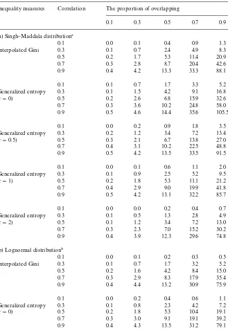
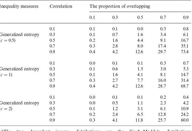
Table 1 reports the (average) simulation results of the 100 runs for the Singh}Maddala and the lognormal distributions, respectively. For each distri-bution, we conduct simulations for"ve inequality indices (the interpolated Gini and four generalized entropy measures corresponding to c"0, 0.5, 1 and 2). The number at the intersection of each correlation level and each overlapping level indicates the average percentage increase in the standard error of*GK Ior
*¹K cif sample dependency is ignored. That is, each number is the average of the percentage di!erences, [(uncorrected standard error!corrected standard error)/corrected standard error]]100, from the 100 runs. For example, the number 88.1 (at the intersection of 0.9 coe$cient of correlation and 0.9 overlap-ping for the interpolated Gini in Table 1a) means that, on average, the standard error would go up by 88.1% if sample dependency is not taken into account.
Table 1
Simulation studies: increases in standard errors if sample dependency is not corrected Inequality measures Correlation The proportion of overlapping
0.1 0.3 0.5 0.7 0.9
(a) Singh}Maddala distribution!
0.1 0.0 0.1 0.4 0.9 1.3
Interpolated Gini 0.3 0.1 0.7 2.4 4.9 8.3
0.5 0.2 1.7 5.3 11.4 20.9
0.7 0.3 2.8 8.7 20.4 42.6
0.9 0.4 4.2 13.3 33.3 88.1
0.1 0.1 0.7 1.7 3.3 5.2
Generalized entropy (c"0)
0.3 0.1 1.5 4.2 9.1 16.8
0.5 0.2 2.6 6.8 15.9 32.6
0.7 0.3 3.6 10.2 24.8 58.0
0.9 0.5 4.6 14.4 35.6 105.5
0.1 0.0 0.2 0.9 1.8 3.5
Generalized entropy (c"0.5)
0.3 0.2 1.2 3.4 7.2 13.4
0.5 0.3 2.1 6.7 13.8 27.0
0.7 0.4 3.1 10.2 22.5 48.8
0.9 0.5 4.2 13.5 33.5 91.5
0.1 0.0 0.1 0.6 1.1 2.0
Generalized entropy (c"1)
0.3 0.1 0.9 2.5 5.2 9.5
0.5 0.2 1.8 5.3 11.1 21.2
0.7 0.4 2.9 9.0 19.9 41.8
0.9 0.5 4.2 13.1 32.2 85.7
0.1 0.0 0.0 0.2 0.4 0.7
Generalized entropy (c"2)
0.3 0.1 0.5 1.3 2.8 4.9
0.5 0.1 1.2 3.4 7.2 13.0
0.7 0.3 2.3 7.0 15.2 30.2
0.9 0.4 3.9 12.3 29.6 74.8
(b) Lognormal distribution"
0.1 0.0 0.1 0.2 0.3 0.5
Interpolated Gini 0.3 0.1 0.7 1.7 3.2 5.2
0.5 0.2 1.6 4.2 8.4 15.0
0.7 0.3 2.9 8.3 17.9 35.4
0.9 0.4 4.4 13.2 30.9 75.9
0.1 0.0 0.2 0.4 0.6 1.1
Generalized entropy (c"0)
0.3 0.1 0.8 2.3 4.2 7.2
0.5 0.2 1.8 5.3 10.4 19.1
0.7 0.3 3.0 9.1 19.1 39.2
Table 1 (continued)
Inequality measures Correlation The proportion of overlapping
0.1 0.3 0.5 0.7 0.9
0.1 0.1 0.1 0.0 0.3 0.8
Generalized entropy (c"0.5)
0.3 0.1 0.7 1.6 3.4 6.1
0.5 0.2 1.6 4.4 9.1 16.7
0.7 0.3 2.8 8.0 17.4 35.1
0.9 0.4 4.2 12.6 29.7 73.4
0.1 0.0 0.1 0.1 0.3 0.7
Generalized entropy (c"1)
0.3 0.1 0.6 1.5 3.0 5.3
0.5 0.1 1.6 4.1 8.1 14.7
0.7 0.3 2.7 7.7 16.0 31.4
0.9 0.4 4.2 12.6 28.7 68.7
0.1 0.0 0.1 0.1 0.2 0.4
Generalized entropy (c"2)
0.3 0.0 0.5 1.1 2.3 4.2
0.5 0.1 1.2 3.1 6.1 10.9
0.7 0.2 2.4 6.5 12.8 24.2
0.9 0.3 4.1 11.8 25.7 60.0
!The two dependent income distributions are the Singh}Maddala distributions
SM(1.6971, 8.3679). The pseudo-random numbers are generated using the routine provided in Microsoft FORTRAN90. The sample size of each simulation is 5000 and each simulation is repeated 100 times. All increases are represented in percentage and are calculated as the average of the di!erences, [(uncorrected standard error!corrected standard error)/corrected standard error]]100, from the 100 runs.
"The two dependent income distributions are lognormal distributions with mean 10 000 and standard deviation 5000. The pseudo-random numbers are generated using the routine provided in Microsoft FORTRAN90. The sample size of each simulation is 5000 and each simulation is repeated 100 times. All increases are represented in percentage and are calculated as the average of the di!erences, [(uncorrected standard error!corrected standard error)/corrected standard error]]100, from the 100 runs.
thep-value will be changed. Of course, if only a few signi"cance levels such as 0.01, 0.05 and 0.10 are used, as we usually do in empirical studies, it is possible that the correction for sample dependency may not change the signi"cance level of a given di!erence.
4.2. Applications to the CPS and PSID data
partially dependent samples and the PSID data is an example of completely dependent samples. The CPS sample rotates every 2 years and, by design, about half of the households are overlapping (see the CPS website at http://www.bls.census.gov/cps). Considering, however, that some people may move out of their dwellings every year and that some may not respond to the survey, the actual overlap is closer to 40%. The PSID is longitudinal and all individuals are re-interviewed every year and thus the proportion of overlapping in theory is 100%.
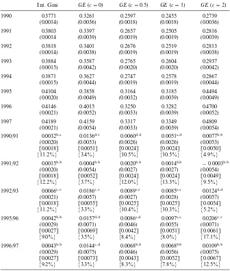
Table 2 reports results on annual U.S. family income inequality and its changes from 1990 to 1997. We include in our sample all primary families and subfamilies but exclude all people living in group quarters; we also drop all entries with zero or negative family incomes in order to use the generalized entropy class of inequality. The top half of the table provides estimates of inequality indices (interpolated Gini index and four generalized entropy measures) and the associated standard errors (inside parentheses). The bottom half documents the inequality comparisons of consecutive years. In each cell there are four numbers: the change in the inequality index; the standard error of the inequality changewithoutcorrecting for sample dependency (inside paren-theses); the standard error with correction for sample dependency (inside brackets); the percentage increase in the standard error if sample dependency is not corrected (inside braces). Consider, for example, the comparison of the Gini coe$cient between 1990 and 1991. The"rst number (0.0032) is the di!erence between 1991's Gini index and 1990's Gini index, the second number (0.0020) is the standard error of the Gini di!erence without correcting for sample depend-ency, the third number [0.0018] is the standard error of the Gini di!erence with correction for sample dependency, the fourth number M11.2%N re#ects the percentage increase in the standard error (from 0.0018 to 0.0020) if sample dependency is not corrected.
Table 2
U.S. family income inequality: 1990}1997 (CPS data)!
Int. Gini GE(c"0) GE(c"0.5) GE(c"1) GE(c"2)
1990 0.3771 0.3261 0.2597 0.2455 0.2739
(0.0014) (0.0036) (0.0018) (0.0018) (0.0036)
1991 0.3803 0.3397 0.2657 0.2505 0.2816
(0.0014 (0.0039) (0.0019) (0.0019) (0.0039)
1992 0.3818 0.3401 0.2676 0.2519 0.2813
(0.0014) (0.0038) (0.0019) (0.0019) (0.0038)
1993 0.3884 0.3587 0.2765 0.2604 0.2937
(0.0015) (0.0042) (0.0020) (0.0020) (0.0042)
1994 0.3871 0.3627 0.2747 0.2578 0.2867
(0.0015) (0.0044) (0.0019) (0.0019) (0.0044)
1995 0.4104 0.3858 0.3164 0.3185 0.4494
(0.0020) (0.0049) (0.0032) (0.0039) (0.0049)
1996 0.4146 0.4015 0.3250 0.3282 0.4700
(0.0021) (0.0052) (0.0033) (0.0039) (0.0052)
1997 0.4189 0.4159 0.3317 0.3349 0.4809
(0.0021) (0.0054) (0.0033) (0.0039) (0.0054)
1990/91 0.0032",# 0.0136$,% 0.0060$,$ 0.0051#,$ 0.0077","
(0.0020) (0.0053) (0.0026) (0.0026) (0.0053)
[0.0018] [0.0051] [0.0024] [0.0024] [0.0050]
M11.2%N M3.4%N M10.5%N M10.5%N M4.9%N
1991/92 0.0015"," 0.0004"," 0.0020"," 0.0014"," !0.0003","
(0.0020) (0.0054) (0.0027) (0.0027) (0.0054)
[0.0018] [0.0052] [0.0024] [0.0024] [0.0049]
M12.2%N M3.7%N M12.0%N M13.3%N M9.5%N
1992/93 0.0066%,% 0.0186%,% 0.0089%,% 0.0085%,% 0.0124$,$
(0.0021) (0.0057) (0.0027) (0.0028) (0.0057)
[0.0018] [0.0055] [0.0025] [0.0025] [0.0054]
M11.2%N M3.3%N M10.4%N M10.3%N M5.2%N
1995/96 0.0042"," 0.0157$,$ 0.0086#,$ 0.0097#,# 0.0206%,%
(0.0029) (0.0071) (0.0046) (0.0055) (0.0071)
[0.0027] [0.0069] [0.0042] [0.0051] [0.0061]
M9.0%N M3.5%N M8.4%N M8.0%N M17.1%N
1996/97 0.0043"," 0.0144#,$ 0.0068"," 0.0068"," 0.0109","
(0.0029) (0.0075) (0.0046) (0.0056) (0.0075)
[0.0027] [0.0073] [0.0043] [0.0052] [0.0067]
M9.2%N M3.3%N M8.3%N M7.8%N M12.5%N
!The top half of the table shows the inequality index and the associated standard error (in parentheses). The bottom half shows the di!erence between 2 years'inequality indices; the number in ( ) is the uncorrected standard error of this di!erence (in parentheses); the corrected standard error (in brackets); the percentage di!erence of the correction in the standard error [(uncorrec-ted!corrected)/corrected]]100 (in braces). The"rst symbol on the shoulder of each di!erence indicates signi"cance with the uncorrected standard error while the second symbol indicates signi"cance with the corrected standard error.
"Indicates insigni"cance at the 10% level.
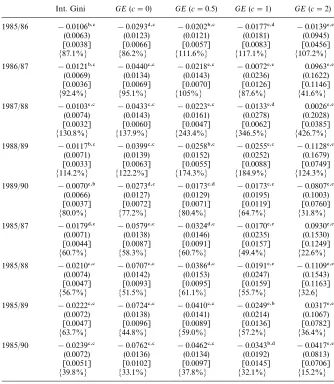
Table 3
U.S. personal earnings inequality: 1985}1990 (PSID data)!
Int. Gini GE(c"0) GE(c"0.5) GE(c"1) GE(c"2) 1985/86 !0.0106",# !0.0293$,# !0.0202",# !0.0177%,$ !0.0139%,%
(0.0063) (0.0123) (0.0121) (0.0181) (0.0945)
[0.0038] [0.0066] [0.0057] [0.0083] [0.0456]
M87.1%N M86.2%N M111.6%N M117.1%N M107.2%N
1986/87 !0.0121",# !0.0440#,# !0.0218%,# !0.0072%,% 0.0963%,%
(0.0069) (0.0134) (0.0143) (0.0236) (0.1622)
[0.0036] [0.0069] [0.0070] [0.0126] [0.1146]
M92.4%N M95.1%N M105%N M87.6%N M41.6%N
1987/88 !0.0103%,# !0.0433#,# !0.0223%,# !0.0133%,$ 0.0026%,%
(0.0074) (0.0143) (0.0161) (0.0278) (0.2028)
[0.0032] [0.0060] [0.0047] [0.0062] [0.0385]
M130.8%N M137.9%N M243.4%N M346.5%N M426.7%N
1988/89 !0.0117",# !0.0399#,# !0.0258",# !0.0255%,# !0.1128%,%
(0.0071) (0.0139) (0.0152) (0.0252) (0.1679)
[0.0033] [0.0063] [0.0055] [0.0088] [0.0749]
M114.2%N M122.2%] M174.3%N M184.9%N M124.3%N
1989/90 !0.0070%," !0.0273$,# !0.0173%,$ !0.0173%,% !0.0807%,%
(0.0066) (0.0127) (0.0129) (0.0195) (0.1003)
[0.0037] [0.0072] [0.0071] [0.0119] [0.0760]
M80.0%N M77.2%N M80.4%N M64.7%N M31.8%N
1985/87 !0.0179$,# !0.0579#,# !0.0324$,# !0.0170%,% 0.0930%,%
(0.0071) (0.0138) (0.0146) (0.0235) (0.1530)
[0.0044] [0.0087] [0.0091] [0.0157] [0.1249]
M60.7%N M58.3%N M60.7%N M49.4%N M22.6%N
1985/88 !0.0210#,# !0.0707#,# !0.0386$,# !0.0191%,% !0.1109%,%
(0.0074) (0.0142) (0.0153) (0.0247) (0.1543)
[0.0047] [0.0093] [0.0095] [0.0159] [0.1163]
M56.7%N M51.5%N M61.1%N M55.7%N M32.6N
1985/89 !0.0222#,# !0.0724#,# !0.0410#,# !0.0249%," 0.0317%,%
(0.0072) (0.0138) (0.0141) (0.0214) (0.1067)
[0.0047] [0.0096] [0.0089] [0.0136] [0.0782]
M63.7%N M44.8%N M59.0%N M57.2%N M36.4%N
1985/90 !0.0239#,# !0.0762#,# !0.0462#,# !0.0343",$ !0.0417%,%
(0.0072) (0.0136) (0.0134) (0.0192) (0.0813)
[0.0051] [0.0102] [0.0097] [0.0145] [0.0706]
M39.8%N M33.1%N M37.8%N M32.1%N M15.2%N
!Each cell shows the di!erence between 2 years'inequality indices; the uncorrected standard error of this di!erence (in parentheses); the corrected standard error (in brackets); the percentage di!erence of the correction in the standard error [(uncorrected!corrected)/corrected]]100 (in braces). The
"rst symbol on the shoulder of each di!erence indicates signi"cance with the uncorrected standard error while the second symbol indicates signi"cance with the corrected standard error. The top half of the table provides comparison of adjacent years between 1985 and 1990 while the bottom half compares 1985 with 1987}1990.
"Indicates signi"cance at the 10% level.
#Indicates signi"cance at the 1% level.
of correction for the generalized entropy index withc"0 for the comparison between 1996 and 1997 changes the signi"cance level; the large 12.5% for the generalized entropy index withc"2 for the same comparison does not change the signi"cance level. This happens because the "rst change in inequality (0.0144) is close to be signi"cant at the 5% level and only a small reduction in the standard error is su$cient to make it signi"cant, but the second change in inequality (0.0109) is far from being signi"cant at the 10% level and even a large reduction in the standard error is not enough to make it signi"cant. It follows that the correction for sample dependency is particularly important and neces-sary if thep-value with uncorrected standard error is already in the neighbor-hood of being signi"cant.
Table 3 compares U.S. personal earnings inequality from 1985 to 1990. The top half of the table reports "ve comparisons of consecutive years while the bottom half compares 1985 with other years (1987}1990). All numbers carry the same meanings as those in Table 2 (bottom half ). In this illustration, we are interested in changes in earnings inequality of those who were employed, thus we limit our samples to those individuals who worked full time and have positive earnings in both years of each comparison. The e!ect of the correction on standard errors varies widely, ranging from 15.2% (the generalized entropy index with c"2 for the 1985/1990 comparison) to 426.7% (the generalized entropy index with c"2 for the 1987/1988 comparison). These corrections a!ect the signi"cance level in 15 of the 25 cases in the top half of the table.
5. Summary and conclusion
Researchers often encounter sample dependency when testing inequality changes across time. Commonly used income samples such as the CPS and PSID are dependent in that they have an overlap in consecutive years. Since conventional inference procedures assume independence among samples, a method of correction for sample dependency is needed.
This paper provided appropriate inference procedures to test the (interpo-lated) Gini coe$cient and the generalized entropy class with dependent samples. We"rst showed that the estimated changes in inequality indices with completely dependent samples have asymptotic normal distributions and that standard errors can be straightforwardly estimated. We then modi"ed the procedure to adjust the standard errors for inequality comparisons with partially dependent samples. The asymptotic covariance of the partially dependent samples can be easily calculated using a two-step procedure.
substantial impacts on standard errors. We also empirically investigated this issue by testing changes in U.S. family income inequality from 1990 to 1997 (using the CPS data) and personal earnings inequality from 1985 to 1990 (using the PSID data). Our empirical results further demonstrated the importance of adjusting standard errors for sample dependency.
While we focused on testing cross-time inequality changes, the method of correction for sample dependency is also applicable to testing marginal changes in inequality. Marginal changes in income inequality refer to the increase or decrease in income inequality of the same population after the population has experienced a change in income. An example of marginal changes is the e!ect of income transfer programs on income distribution. In the United States, a sizable portion of GNP is spent annually on various welfare programs such as food stamps and temporary assistance to needy families (formerly aid to families with dependent children). This has a!ected the income distribution. While re-searchers have generally agreed that welfare programs reduce both income inequality and poverty (see Danziger et al., 1981), they have not arrived at a consensus regarding the magnitude of the reduction. With the social welfare system under scrutiny and in the midst of reforms, accurately measuring the impact of welfare reforms on income inequality is important. Other interesting examples of marginal changes in income inequality include the e!ect of taxation on income inequality and the e!ect of wives'participation in the labor force on family income inequality. The two samples of before- and after-event needed to address these issues are completely dependent and the method proposed in this paper should be used to correct for sample dependency. As we have demon-strated here, failure to use such a method may lead to erroneous conclusions.
Acknowledgements
We thank three anonymous referees, an Associate Editor, Professor Arnold Zellner, Dr. Fanhui Kong, Dr. John Bishop and Professor Ram Shanmugam for useful comments and suggestions on earlier versions of the paper. We are also grateful to Xuemei (Alice) Du for her assistance in computer programming. The usual caveats apply.
References
Aghevli, B., Mehran, F., 1981. Optimal grouping of income distribution data. Journal of the American Statistical Association 76, 22}26.
Aitchison, J., Brown, J., 1969. The Lognormal Distribution with Special References to Its Uses in Economics. Cambridge University Press, Cambridge.
Beach, C., Chaykowski, R., Slotsve, G., 1997. Inequality and polarization of male earnings in the United States, 1968}1990. North American Journal of Economics and Finance 8, 135}151. Bishop, J.A., Formby, J.P., Smith, W.J., 1991a. Lorenz dominance and welfare: changes in the US
distribution of income, 1967}1986. Review of Economics and Statistics 71, 134}139.
Bishop, J.A., Chow, K., Formby, J.P., 1991b. A stochastic dominance analysis of growth, recessions and the US income distribution, 1967}1986. Southern Economic Journal 57, 936}946. Bishop, J.A., Chiou, J., Formby, J.P., 1994. Truncation bias and the ordinal evaluation of income
inequality. Journal of Business and Economic Statistics 12, 123}127.
Bishop, J.A., Formby, J.P., Zheng, B., 1997. Statistical inference and the Sen index of poverty. International Economic Review 38, 381}387.
Bishop, J.A., Formby, J.P., Zheng, B., 1998. Inference tests for Gini-based tax progressivity indexes. Journal of Business and Economic Statistics 16, 322}330.
Cowell, F., 1980. On the structure of additive inequality measures. Review of Economic Studies 47, 521}531.
Cowell, F., 1989. Sampling variance and decomposable inequality measures. Journal of Econo-metrics 42, 27}42.
Danziger, S., Haveman, R., Plotnick, R., 1981. How income transfer programs a!ect work, savings, and the income distribution: a critical review. Journal of Economic Literature 19, 975}1028. Dardanoni, V., Forcina, A., 1997. Inference for the Lorenz Curve Ordering. Mimeo, University of
California at San Diego.
Davidson, R., Duclos, J., 1997. Statistical inference for the measurement of incidence of taxes and transfers. Econometrica 65, 1453}1465.
Formby, J.P., Smith, W.J., Zheng, B., 1999. The coe$cient of variation, stochastic dominance and inequality: a new interpretation. Economics Letters 62, 319}323.
Gail, M., Gastwirth, J.L., 1978. A scale-free goodness-of-"t test for the exponential distribution based on the Lorenz curve. Journal of the American Statistical Association 73, 787}793. Gastwirth, J.L., 1971. A general de"nition of the Lorenz curve. Econometrica 39, 1037}1039. Gastwirth, J.L., 1972. The estimation of the Lorenz curve and Gini index. Review of Economics and
Statistics 54, 306}316.
Gastwirth, J.L., 1974. Large sample theory of some measures of income inequality. Econometrica 42, 191}196.
Gastwirth, J.L., Gail, M., 1985. Simple asymptotically distribution-free methods for comparing Lorenz curves and Gini indices obtained from complete data. In: Basmann, R.L., Rhodes Jr., G.F. (Eds.), Advances in Econometrics, Vol. 4. JAI Press, Connecticut.
Goldie, C., 1977. Convergence theorems for empirical Lorenz curves and their inverses. Advances in Applied Probability 9, 765}791.
Hoe!ding, W., 1948. A class of statistics with asymptotically normal distribution. Annals of Mathematical Statistics 19, 293}325.
Johnson, M., 1987. Multivariate Statistical Inference. McGraw-Hill, New York. Kendall, M., Stuart, A., 1977. The Advanced Theory of Statistics. Macmillan, New York. Lawrance, A., Lewis, P., 1983. Simple dependent pairs of exponential and uniform random variables.
Operations Research 31, 1179}1197.
Lewis, P., Orav, E., 1989. Simulation Methodology for Statisticians, Operations Analysts, and Engineers. Wadsworth & Brooks, Paci"c Grove, CA.
McDonald, J., 1984. Some generalized functions for the size distribution of income. Econometrica 52, 647}663.
Rao, C.R., 1965. Linear Statistical Inference and Its Applications. Wiley, New York. Sen, A., 1973. On Economic Inequality. Clarendon Press, Oxford.
Ser#ing, R.J., 1980. Approximation Theorems of Mathematical Statistics. Wiley, New York. Shorrocks, A., 1980. The class of additively decomposable inequality measures. Econometrica 48,
Singh, S., Maddala, G., 1976. A function for size distribution of incomes. Econometrica 44, 963}970. Schluter, C., 1996. Income distribution and inequality in Germany: evidence from panel data.
STICERD Working Paper, London School of Economics.
Thistle, P., 1990. Large sample properties of two inequality indices. Econometrica 58, 725}728. Zheng, B., 1996. Statistical inferences for testing marginal changes in Lorenz and generalized Lorenz
curves. Mimeo, University of Colorado at Denver.