*Corresponding author.
E-mail address:[email protected] (A. Kimms).
Lot sizing and scheduling with sequence-dependent setup costs
and times and e
$
cient rescheduling opportunities
Knut Haase, Alf Kimms*
Institut fu(r Betriebswirtschaftslehre, Christian Albrechts University of Kiel, Olshausenstr. 40, 24118 Kiel, Germany Received 15 October 1998; accepted 17 August 1999
Abstract
This paper deals with lot sizing and scheduling for a single-stage, single-machine production system where setup costs and times are sequence dependent. A large-bucket mixed integer programming (MIP) model is formulated which considers only e$cient sequences. A tailor-made enumeration method of the branch-and-bound type solves problem instances optimally and e$ciently. The size of solvable cases ranges from 3 items and 15 periods to 10 items and 3 periods. Furthermore, it will become clear that rescheduling can neatly be done. ( 2000 Elsevier Science B.V. All rights reserved.
Keywords: Lot sizing; Scheduling; Production planning and control; Rescheduling; Sequence-dependent setup times
1. Introduction
For many production facilities the expenditures for the setups of a machine depend on the sequence
in which di!erent items are scheduled on the
ma-chine. Especially when a machine produces items of
di!erent family types setups between items of di!
er-ent families are substantially more costly and time consuming than setups between items of the same family. In such a case a just-in-time philosophy will cause frequent setups, i.e. large total setup costs and long total setup times. To reduce the expenditures for the setups items may be produced in lots which satisfy the demand of several periods. The amount of a production quantity in a period which will be used to satisfy demand in later periods must then be
held in inventory. This incurs holding costs. There-fore, we have to compute a schedule in which the sum of setup and holding costs is minimized. In the case of sequence-dependent setup costs the calcu-lation of the setup costs requires the computation of the sequence in which items are scheduled, i.e. we have to consider sequencing and lot sizing simulta-neously.
Despite its relevance only little research has been done in the area of lot sizing and scheduling with sequence-dependent setups. Some papers have been published which are related to the so-called discrete lot sizing and scheduling problem [4], denoted as DLSP. In the DLSP the planning horizon is divided into a large number of small periods (e.g. hours, shifts, or days). Furthermore, it is assumed that the production process always runs full periods without changeover and the setup state is
not preserved over idle time. Such an`
all-or-noth-ingapolicy implies that at most one item will be
produced per period. In [1] a DLSP-like model with sequence-dependent setup costs was
con-sidered "rst. For the DLSP with
sequence-depen-dent setup costs (DLSPSD) an exact algorithm is presented in [2]. There the DLSPSD is trans-formed into a traveling salesman problem with time windows which is then used to derive lower bounds as well as heuristic solutions. An exact solution method for the DLSP with sequence-de-pendent setup costs and times (DLSPSDCT) is proposed in [3]. The optimal enumeration method proposed by [4] is based on the so-called batch sequencing problem (BSP). It can be shown that the BSP is equivalent to the DLSPSDCT for a re-stricted class of instances. The solution methods for the DLSPSDCT and the BSP require large
work-ing spaces, e.g. for instances with six items and"ve
demands per item a working space of 20 megabytes is required. Recently, another new type of model has been published which is called the proportional lot sizing and scheduling problem (PLSP) [5]. The PLSP is based on the assumption that at most one setup may occur within a period. Hence, at most
two items are producible per period. It di!ers from
the DLSP regarding the possibility to compute continuous lot sizes and to preserve the setup state over idle time. A regret-based sampling method is proposed to consider sequence-dependent setup costs and times. In [6] an uncapacitated lot-sizing problem with sequence-dependent setup costs is considered. A heuristic for a static, i.e. constant demand per period, lot-scheduling problem with sequence-dependent setup costs and times is intro-duced in [7]. In [8] the so-called capacitated lot-sizing problem with sequence-dependent setup costs (CLSD) is presented. As in the PLSP, the setup state can be preserved over idle time. But in contrast to the DLSP and PLSP many items are producible per period. Hence, the DLSP and PLSP are called small-bucket problems and the CLSD is a large-bucket problem. For a review of lot-sizing and scheduling models we refer to [5]. A large-bucket problem with sequence-dependent setup costs and times is not considered in the literature so far. In this paper we will close this gap.
The text is organized as follows: in the next
section we brie#y describe the practical
back-ground that inspired our work on this subject. In
Section 3, we give a mathematical formulation of the problem under concern. Afterwards, reschedul-ing is discussed in Section 4. In Section 5, an
opti-mal enumeration method is outlined. The e$ciency
of the algorithm is tested by a computational study in Section 6.
2. A real-world case
Linotype-Hell AG, Kiel (Germany), manufac-tures high technology machines for the setting and printing business. A case study coauthored by one of the authors and provided in [9] informally describes the situation up to 1995 as follows. Although a commercial Siemens software package already is in use for production planning and con-trol, demands are usually not met right in time. A milling machine, a so-called BZV07-2000,
is identi"ed as being the bottleneck. Hence,
one searches for alternatives out of this situation. Buying an additional milling machine is considered to be too expensive. And using outside capacities is not wanted, because the know-how should be
kept inside the "rm. Hence, one of the authors
suggests using the available capacity of the milling
machine more e$ciently by improved production
planning.
The production planning problem for the milling machine indeed is a lot-sizing and scheduling prob-lem with sequence-dependent setups. Setting the milling machine up actually means to load a
speci-"c program into memory that runs the numerically
controlled milling machine, and to mount speci"c
tools and holders. The sequence-dependent setup
time consists of taking o!tools and holders,
load-ing another program, and mountload-ing other tools and holders. The shortcoming of the planning soft-ware already in use is that average data for setup times are used as input for planning, and sequence dependencies are not considered. But, in practice, total setup times result from planning. As a conse-quence, the idea is near to formulate and to solve a model for this particular problem.
our contact persons were busy with this project since then.
3. A mixed-integer programming formulation
In this section we introduce the lot-sizing and scheduling-problem with sequence-dependent setup costs and times, denoted as LSPSD. Before we present a mathematical formulation of the LSPSD we have to give the underlying assumptions and
have to introduce some de"nitions.
Assumption 1. The setup state is kept up over idle time.
We point out this simple fact because in the DLSP (cf. [3,10]) it is assumed that the setup state is lost after idle time. Only a few practical applica-tions seem to require the loss of the setup state. This is emphasized by the fact that Assumption 1 is also
made in a wide variety of di!erent lot-sizing and
scheduling models (cf. [5]).
We consider a large-bucket problem. This is to say that more than one item can be produced per period (e.g. per week).
Now, let sc
i,j (sti,j) denote the setup cost (setup
time) for a setup from itemito itemj. We compute
setup costs as follows:
Assumption 2. Setup cost has the form
sc
i,j"fj#f4#sti,jwherefjare"xed cost andf4#are
opportunity cost per unit of setup time.
In [2] instances are considered where the
tri-angle inequality for the setup costs is not ful"lled.
For practical purposes this seems to be not a very important case. Hence, we exclude such solutions by the following assumption:
Assumption 3. Setup times satisfy the triangle in-equality, i.e. st
i,j)sti,k#stk,jfor alli,j,k"1,2,J,
whereJis the number of di!erent items to be
con-sidered.
Due to assumption 2 the triangle inequality is also valid for the setup costs.
Corollary 4. For each item at most one lot will be produced in a period.
Note, Corollary 4 is underlying the classical un-capacitated and un-capacitated lot-sizing problems (cf. e.g. [6]), too.
Furthermore, we assume the following:
Assumption 5. If the production of an item starts in a period then the inventory of the item must be empty at the end of the previous period.
Assumption 6. Each setup will be performed within a period.
De5nition 7. The ordered set seq(n):"(i
1,2,ik,
2,iMn) denotes a sequencenofMn di!erent items
within a period wherei
1(ik,iMn) is said to be the"rst
(kth, last) item of seq(n).
seq(n) is a sequence in which some items can be
(e$ciently) scheduled where it needs to be de"ned
what e$cient really means.
De5nition 8. The setup cost (setup time) of the
se-quence seq(n) is given by SC
n"+Mj/1n~1scij,ij`1 (ST
n"+Mj/1n~1stij,ij`1).
E$ciency can now be de"ned as follows:
De5nition 9. Consider two feasible sequences seq(n)
and seq(n{)with (i1,2,i
Mn), and (i@1,2,i@Mn{),
respec-tively. seq(n) dominates seq(n{) if SC
n(SCn{,
i
1"i@1,iMn"iMn{, and seq(n{)consists exactly of the
same items as seq(n). seq(n) is called e$cient if there
exists no other sequence seq(nA)that dominates seq(n).
Note, the computation of an e$cient sequence is
a traveling salesman problem (TSP) in which the
salesman starts at&custom'i
1 and stops at&custom'
i
Mn. Nowadays, optimal solution procedures for the
TSP which work in reasonable time with hundreds of customers exist. In the following we need to
con-sider only e$cient sequences.
feasible sequences. This will turn out to be important for rescheduling.
Before we give a MIP-model formulation to
de"ne the problem at hand precisely, let us
introduce some notation.
Parameters
J the number of di!erent items
N the total number of e$cient sequences
¹ the number of periods
A
j the set of indices which are associated toe
$cient sequences which contain itemj, i.e.
A
j"Mn3M1,2,NN Dj3seq(n)N
B big number; e.g.B*maxM+Tt/1d
j,tDj"1,2,JN
C
t the capacity available in periodt
d
j,t the demand for itemjat the end of periodt
F
j the set of indices which are associatedto e
$cient sequences in which itemjis
scheduled as the"rst item, i.e.
F
j"Mn3M1,2,NN Dseq(n)"(j,2,iMn)N
h
j holding cost which is incurred to hold oneunit of itemjat the end of a period in inven-tory
¸
j the set of indices which are associatedto e
$cient sequences in which itemjis
sched-uled as the last item, i.e. ¸
j"Mn3M1,2,NN Dseq(n)"(i1,2,j)N
p
j capacity needs for producing one unit of itemj
SC
n setup cost which is incurred for schedulingsequencen
ST
n setup time which is required to schedule se-quencen
Decisionvariables
I
j,t the inventory of item(I jat the end of periodt
j,0"0 without loss of generality)
q
j,t the quantity of itemodt jto be produced in
peri-S
n,t a binary variable indicating whether sequencenis used in periodt(S n,t"1) or not (Sn,t"0) (an initial setup state is also taken into account, i.e.&n|M1,2,NN:Sn,0"1'Sn{,0"0∀n@On). The LSPSD can now be stated as follows:
Problem LSPSD The objective function (1) determines the total setup and holding costs. Constraints (2) are the inventory balances. Constraint (3) states that for each period we have to choose exactly one se-quence in which items are scheduled. By constraint (4) we satisfy that the setup state is preserved be-tween two adjacent periods. Constraint (5) ensures that an item can only be produced in a period if the machine is setup for it. Constraint (6) guarantees that a new lot is scheduled for an item only if the inventory is empty (zero-switch-property). Con-straints (7) are the capacity conCon-straints. These con-straints also include that all setups are done within a period completely, i.e. no setup is performed over a period border. The last two constraints, (8) and
(9), properly de"ne the domains of the binary and
Table 2
Item speci"c sets of sequence indices
j A
Sequences and associated setup costs and times
n seq(n) ST
For example, let S
1,0"1, Sn,0"0 for n'1,
¹"4, J"3, (h
j)"(1, 1, 2), (pj)"(2, 1, 1),
(C
t)"(100, 100, 100, 100), and
(d
(e$cient) sequences and the associated setup times
and costs as given in Table 1. The item speci"c sets
A
j, Fj, and¸j are provided in Table 2. Note, to
keep the example small and clear we have chosen
J"3 and thus Table 1 contains all possible
se-quences. If we had J"4, then for example either
the sequence (1, 2, 3, 4) or (1, 3, 2, 4), but not both,
would have to be considered as an e$cient
se-quence. Note, if both sequences are e$cient, we can
choose one of them arbitrarily.
The optimal solution, computed with a standard
solver, is ZH"585. The associated production
quantities and non-zero binary decision variables are
In the solution itemj"2 is scheduled as the last
item in periodt"1 and as"rst item in periodt"2
which allows "ve units of the demand d
2,2 to be
produced in period t"1. This is necessary, since
the capacity in periodt"2 is completely used up
for setups and production (ST
7#+3j/1pjqj,2"
5#2]10#1]75"100"C
2).
4. Rescheduling
Now, we will show how rescheduling (cf. [11]) can easily be integrated into the LSPSD. Let us
assume that new information } due to customer
requests}result in changes of the demand matrix
Table 3
Outline of the enumeration in periodt
Step 0: Compute SEQ t.
Step 2: Choose seq
t"(i1,2,ikt)3SEQt.
Step 3: SEQ
t:"SEQt!MseqtN.
Step 4: Set cost
t"SC(seqt)#+Jj/1(CDj,t!dj,t)hj#costt`1.
Step 5: Computeq
j,t(j"1,2,J).
Step 6: If`not boundago to periodt!12
N
backtracking to periodt#1.
Therefore, we de"ne
SEQ
t the set of sequences which are allowed tobe scheduled in periodt, and
q&
j,t the minimum production quantity of itemwhich has to be scheduled in periodt. Note,j
q&
and update the capacities usingC@
t"Ct!+jJ/1pjq&j,t for t"1,2,¹ the LSPSD is extended for re-scheduling.
In summary we"nd out that rescheduling equals
the scheduling process but reduces the solution space when compared with the original instance. Rescheduling therefore needs less computational
e!ort than"nding a"rst schedule (unless we extend
the planning horizon).
5. A fast enumeration scheme
To "nd an optimal solution for a particular
LSPSD instance we must "rst note that once
we have "xed all the binary variables S
n,t in the MIP-formulation above, the remaining sub-problem is an LP-sub-problem. In other words,
enu-merating all the ¹-tuples (seq
1,2, seqT) where
seq
t denotes the sequence chosen in periodt, and
solving the corresponding LP-problem then, will reveal the optimal solution. Unfortunately,
the number of ¹-tuples is quite large, ((J!1)
2(J~2)#1)Tto be precise.
Hence, we need a more sophisticated approach to tackle this problem. In its essence, the procedure that we propose is a branch-and-bound (B&B)
method. Roughly speaking, we start in period ¹,
perform a branching step by choosing seq
T, and
then move on to period one step by step doing backtracking in-between if necessary.
To provide more details, we use the following notation: If seq
tis a sequence of the form (i1,2,ikt)
wherek
t*1, then,"rst (seqt)"i1and last(seqt)"ikt
are the"rst and the last item, respectively, in seq
t.
remaining demand for item j in period t. Note,
initially we haveq
j,t"0 for all itemsjin all periods
t. Furthermore, let SEQ
t be the set of all e$cient
sequences to be considered in periodt.
Now, we are ready to describe the solution scheme (see Table 3) in more detail.
Some things need to be discussed. First, inStep 0,
SEQ
t can of course be chosen as the set of all
sequences. But, we can eliminate all those se-quences which contain items with a zero cumulat-ive demand. In other words, items for which no demand occurs, need not be produced. The only exception from that is that the last item in a
se-quence must equal the"rst item in seq
t`1sequence,
i.e. last(seq
t)""rst(seqt`1) for t"1,2,¹!1. In
addition, SEQ
t must contain only those sequences
to say, that all sequences seq
t contained in SEQt
must ful"ll
Remember, that lots (except the one for the "rst
item in a sequence) must not range over period borders. For rescheduling, the choice of SEQ
t must
be a subset of the valid sequences in periodt.
In Step 2seq
t can be chosen arbitrarily. In our
implementation we choose long sequences before we choose short ones. Ties are broken in lexi-cographical order.
Step 5 directly corresponds to solving a linear program. Due to our assumption that lots (i.e. CD
If period 1 is under concern, we face a feasible solution if and only if the total demand for periods
1 to ¹is equal to the total production of periods
1 to¹ for all itemsj"1,2,J. And, cost1 is the
objective function value for the feasible solution at hand.
Finally, in Step 6 we test if we can prune the
search tree. Two tests are done here. First, we check if the remaining capacity exceeds the capacity de-mand, i.e.
t is the set of items which must be
produced in periods 1,2,t!1 and for which
a setup must occur. Note, only a lower bound of the
setup time is considered here. Second, we test if the current situation is bounded by costs. Assume, that we have an upper bound of the overall problem, say
upperbound. Furthermore assume, that we have
a lower bound of costs, say lowerbound
1,t~1, that
will additionally occur if we schedule sequences in
the periods t!1,2,1. Then, we simply check
cost
t#lowerbound1,t~1*upperbound to prune
the tree.
The e$ciency of our procedure highly depends
on these lower bounds.
Let us discuss the lower bounds only, since the upper bounds are computed using standard
tech-niques (i.e. starting with in"nity we update the
upper bound whenever a feasible solution is found that improves the current best bound). Before we
start trying to solve an instance with Jitems and
¹periods, we cut the horizon at the end and solve
the resulting instance withJ items and the ¹!1
periodst"1,2,¹!1. Following the same lines,
before we solve the¹!1 periods instance we solve
the¹!2 periods instance and so on. Note, that if
a smaller instance is not feasible, the larger cannot be either. In summary we start with an instance of 1 period only which provides the lower bound lowerbound
1,1. Then we solve an instance with
2 periods which gives lowerbound
1,2 and so on
until we are done. The trick here is that we can use the lower bounds computed by solving small in-stances when we solve the large inin-stances. As com-putational studies have shown, the speed-up is dramatic. E.g. running instances with three items and 10 periods of time took more than an hour without these bounds and now terminates after a few seconds.
This bounding scheme is very e$cient in terms of
both, run-time and memory space. While the
for-mer one will be veri"ed in the next section, the
latter one should be evident.
6. Computational study
To test the proposed method we ran a C-imple-mentation on a Power PC computer with 80 MHz measuring run-time performances. A total of 540 instances were systematically generated as follows:
For all items we choose p
Table 4
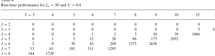
Run-time performance forf
4#"50 and;"0.4
¹"3 4 5 6 7 8 9 10 15 20
J"2 0 0 0 0 0 0 0 0 0 1
J"3 0 0 0 0 0 0 0 0 5 162
J"4 0 0 0 1 2 5 10 39 1966
J"5 0 1 3 12 20 96 173 2052
J"6 2 9 39 83 209 1375 2658
J"7 13 61 181 511 1295
J"8 144 1729
J"9 537
J"10 2428
assumed to be set up for item 1 initially. The
num-ber of items J ranges from 2 to 10 items and the
number of periods¹ranges from 3 to 10, 15, and 20
periods. We then randomly generated an external demand matrix with 10 items (rows) and 20 periods
(columns) where each entryd
j,tis chosen out of the
interval [40,60] with uniform distribution. Hence, this matrix contains no zero values which possibly would reduce the number of sequences to be con-sidered per period. Analogously, a setup time matrix with 10 items is generated where each entry st
i,j (iOj) is randomly chosen out of the
interval [2,10] (and st
j,j"0). The choice of setup times is done so that all triangle inequalities
are ful"lled. Holding costs for 10 items are
random-ly chosen, too, where each value h
j is drawn
out of the interval [2,10] with uniform
distribut-ion. For an instance withJitems and¹periods we
then use the data given in the "rst J rows and
the"rst¹columns of the external demand matrix,
the "rst J rows and columns of the setup time
matrix, and the "rstJ entries of the holding cost
vector. This implements the concept of common random numbers in our tests. The setup cost sc
i,j
for changing the setup state from itemito itemjare
computed by
sc
i,j"f4#sti,j, i,j"1,2,J,
where the parameter f
4# is systematically varied
using f
4#"50 and 500. The capacity per period
C
t is determined according to
C
t"
+Jj/1d
j,t
; , t"1,2,¹,
where the capacity utilization; is systematically
varied using;"0.4, 0.6, and 0.8. Note, the
utiliz-ation of capacity is an estimate only, because setup
times do not a!ect the computation ofC
t. Hence,
a value;"0.8 actually means that the utilization
of capacity by production and setup actions is greater than 80% on average. Note, the more items there are, the more capacity is consumed by setup time. In summary, we have
DM2,2, 10ND]DM3,2, 10, 15, 20ND]DM50, 500ND
DM0.4, 0.6, 0.8ND"540 instances.
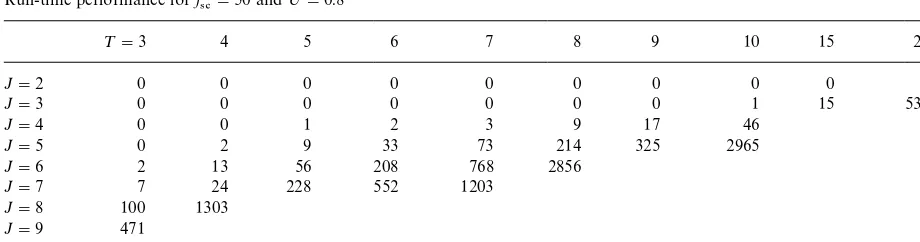
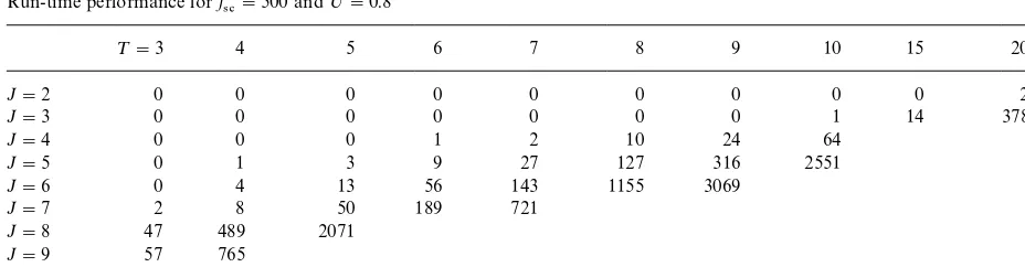
Tables 4}9 provide the run-time results of our
study. All results are given in CPU}seconds. A time
limit of 3600 CPU-seconds is used. Missing entries thus indicate that the corresponding instance can-not be solved optimally within one hour on our platform. Zeroes indicate that the method needs less than 0.5 CPU-seconds to compute the opti-mum solution. The run-times given here do not
include the time needed to compute the e$cient
sequences. This is because in a real-world situation
the number of items J does not change in
the short-term and thus solving the set of travel-ing salesman problems needs to be done once
and for all. The e!ort for doing so can thus be
neglected.
As expected, it turns out that the parameters
Jand ¹do have a signi"cant impact on the
run-time performance. In almost all cases, the run-run-time
grows faster withJthan with¹. For instance, see
Table 4 where the instance withJ"7 and ¹"4
Table 5
Run-time performance forf
4#"50 and;"0.6
¹"3 4 5 6 7 8 9 10 15 20
J"2 0 0 0 0 0 0 0 0 0 1
J"3 0 0 0 0 0 0 0 0 5 136
J"4 0 0 0 1 2 5 9 37
J"5 0 1 2 11 19 93 167 2001
J"6 2 9 38 82 204 1352 2633
J"7 13 60 179 505 1282
J"8 194 2570
J"9 613
J"10
Table 6
Run-time performance forf
4#"50 and;"0.8
¹"3 4 5 6 7 8 9 10 15 20
J"2 0 0 0 0 0 0 0 0 0 1
J"3 0 0 0 0 0 0 0 1 15 530
J"4 0 0 1 2 3 9 17 46
J"5 0 2 9 33 73 214 325 2965
J"6 2 13 56 208 768 2856
J"7 7 24 228 552 1203
J"8 100 1303
J"9 471
J"10
Table 7
Run-time performance forf
4#"500 and;"0.4
¹"3 4 5 6 7 8 9 10 15 20
J"2 0 0 0 0 0 0 0 0 1 8
J"3 0 0 0 0 1 2 4 7 164
J"4 0 0 1 6 20 78 331 732
J"5 0 3 20 125 1560
J"6 1 11 176 1350
J"7 4 153 1581
J"8 39 3501
J"9 201
J"10 2489
¹"4 we measure 1729 CPU-seconds, and for
J"7 and ¹"5 we need 181 CPU-seconds. Varying the setup costs (measured by the
para-meter f
4#) and the capacity utilization; does not
drastically a!ect the order of magnitude of problem
sizes that can be solved within reasonable time. It
Table 8
Run-time performance forf
4#"500 and;"0.6
¹"3 4 5 6 7 8 9 10 15 20
J"2 0 0 0 0 0 0 0 0 0 5
J"3 0 0 0 0 0 1 2 3 175
J"4 0 0 2 6 18 50 118 314
J"5 0 2 15 81 554 2138
J"6 1 18 216 862
J"7 5 134 1580
J"8 49
J"9 247
J"10 2300
Table 9
Run-time performance forf
4#"500 and;"0.8
¹"3 4 5 6 7 8 9 10 15 20
J"2 0 0 0 0 0 0 0 0 0 2
J"3 0 0 0 0 0 0 0 1 14 378
J"4 0 0 0 1 2 10 24 64
J"5 0 1 3 9 27 127 316 2551
J"6 0 4 13 56 143 1155 3069
J"7 2 8 50 189 721
J"8 47 489 2071
J"9 57 765
J"10 826
make instances easier to solve. Compare for in-stance Table 6 with Table 9 where this seems to be the case, whereas a comparison of Table 4 with Table 7 does not give such a proof.
Since we used instances with fully"lled demand
matrices the results can be seen as worst case esti-mates on the run-time performance. Facing instan-ces with sparse demand matriinstan-ces would give shorter run-times, because the number of sequences to be considered within a period decreases. This is due to the fact that items with no cumulative de-mand need not be scheduled and thus sequences containing such items need not be enumerated.
A similar argument applies to the e!ort for
res-cheduling. Since rescheduling means to impose some restrictions on the sequences that are allowed to be scheduled, its run-time will be less than what can be read in the tables.
A benchmark test with the standard solver LINDO gives convincing results. Within 3600
CPU-seconds, LINDO is able to solve the instan-ces with four items and six periods. In contrast to that, our procedure needs less than 6 seconds to give the optimum result.
7. Conclusions
In this paper we proposed a model for lot sizing and scheduling with sequence-dependent setups which was inspired from a practical case at
Lino-type-Hell AG. The key element for the e$ciency of
the method is based on an idea derived from
prob-lem speci"c insights. Roughly speaking, this idea is
that if we know what items to produce in a period but we do not know the lot sizes yet, we can nevertheless determine the sequence in which these items are to be scheduled.
In contrast to other approaches which su!er from
requires modest capacities. This is mainly due to a novel idea for computing lower bounds to prune the search tree. Memorizing partial schedules seems to be avoidable now. Beside the low memory space usage, the lower bounding technique amazes with high speed-ups.
The size of the instances that are solved is of practical relevance as it is proven by case studies in [2] (food industry) and [9] (discrete part manufac-turing) where instances with less than 10 items occur.
Acknowledgements
We are grateful to Andreas Drexl for his steady
support. Also, we thank Ste!en Wernert.
References
[1] L. Schrage, The multiproduct lot scheduling problem, in: M.A.H. Dempster et al. (Eds.), Deterministic and Stocastic Scheduling, Dordrecht/Holland, 1982, pp. 233}244. [2] B. Fleischmann, The discrete lot-sizing and scheduling
problem with sequence-dependent setup-costs, European Journal of Operational Research 75 (1994) 395}404.
[3] M. Salomon, M.M. Solomon, L.N. Van Wassenhove, Y.D. Dumas, S. Dauzere-Peres, Solving the discrete lotsizing and scheduling with sequence dependent set-up costs and set-up times using the Travelling Salesman Problem with time windows, European Journal of Operational Research 100 (1997) 494}513.
[4] C. Jordan, A. Drexl, Lotsizing and scheduling by batch sequencing, Management Science 44 (1998), 698}713. [5] A. Drexl, A. Kimms, Lot sizing and scheduling*survey
and extensions, European Journal of Operational Research 99 (1997) 221}235.
[6] D.M. Dilts, K.D. Ramsing, Joint lot sizing and scheduling of multiple items with sequence dependent setup costs, Decision Sciences 20 (1989) 120}133.
[7] G. Dobson, The cyclic lot scheduling problem with se-quence-dependent setups, Operations Research 40 (1992) 736}749.
[8] K. Haase, Capacitated lot-sizing with sequence dependent setup costs, OR Spektrum 18 (1996) 51}59.
[9] K. Haase, L. GoKpfert, Engpassorientierte Fertigungs-steuerung bei reihenfolgeabhaKngigen RuKstvorgaKngen in einem Unternehmen der Satz- und Drucktechnik, Zeitschrift fuKr Betriebswirtschaft 66 (1996) 1511}1526. [10] D. Cattrysse, M. Salomon, R. Kuik, L.N. Van
Wassen-hove, A dual ascent and column generation heuristic for the discrete lotsizing and scheduling problem with setup-times, Management Science 39 (1993) 477}486.