Table of Contents
6. Regression Analysis
What does entropy have to do with it? The ID3 algorithm
9. Recommender Systems
The MongoDB extension for geospatial databases Indexing in MongoDB
Why NoSQL and why MongoDB? Other NoSQL database systems Summary
11. Big Data Analysis with Java
Java NetBeans MySQL
MySQL Workbench
Accessing the MySQL database from NetBeans The Apache Commons Math Library
The javax JSON Library The Weka libraries MongoDB
Java Data Analysis
Copyright © 2017 Packt Publishing
All rights reserved. No part of this book may be reproduced, stored in a retrieval system, or transmitted in any form or by any means, without the prior written permission of the publisher, except in the case of brief quotations embedded in critical articles or reviews.
Every effort has been made in the preparation of this book to ensure the
accuracy of the information presented. However, the information contained in this book is sold without warranty, either express or implied. Neither the authors, nor Packt Publishing, and its dealers and distributors will be held liable for any damages caused or alleged to be caused directly or indirectly by this book.
Safis Editing
Indexer
Tejal Daruwale Soni
Graphics
Tania Dutta
Production Coordinator
Arvindkumar Gupta
Cover Work
About the Author
John R. Hubbard has been doing computer-based data analysis for over 40 years at colleges and universities in Pennsylvania and Virginia. He holds an MSc in computer science from Penn State University and a PhD in
mathematics from the University of Michigan. He is currently a professor of mathematics and computer science, Emeritus, at the University of Richmond, where he has been teaching data structures, database systems, numerical analysis, and big data.
Dr. Hubbard has published many books and research papers, including six other books on computing. Some of these books have been translated into German, French, Chinese, and five other languages. He is also an amateur timpanist.
About the Reviewers
Erin Paciorkowski studied computer science at the Georgia Institute of Technology as a National Merit Scholar. She has worked in Java
development for the Department of Defense for over 8 years and is also a graduate teaching assistant for the Georgia Tech Online Masters of Computer Science program. She is a certified scrum master and holds Security+,
Project+, and ITIL Foundation certifications. She was a Grace Hopper Celebration Scholar in 2016. Her interests include data analysis and information security.
Alexey Zinoviev is a lead engineer and Java and big data trainer at EPAM Systems, with a focus on Apache Spark, Apache Kafka, Java concurrency, and JVM internals. He has deep expertise in machine learning, large graph processing, and the development of distributed scalable Java applications. You can follow him at @zaleslaw or https://github.com/zaleslaw.
Currently, he's working on a Spark Tutorial at
https://github.com/zaleslaw/Spark-Tutorial and on an Open GitBook about Spark (in Russian) at
https://zaleslaw.gitbooks.io/data-processing-book/content/.
eBooks, discount offers, and more
Did you know that Packt offers eBook versions of every book published, with PDF and ePub files available? You can upgrade to the eBook version at
www.PacktPub.com and as a print book customer, you are entitled to a discount on the eBook copy. Get in touch with us at
<customercare@packtpub.com> for more details.
At www.PacktPub.com, you can also read a collection of free technical articles, sign up for a range of free newsletters and receive exclusive discounts and offers on Packt books and eBooks.
https://www.packtpub.com/mapt
Get the most in-demand software skills with Mapt. Mapt gives you full
Why subscribe?
Fully searchable across every book published by Packt Copy and paste, print, and bookmark content
Customer Feedback
Thanks for purchasing this Packt book. At Packt, quality is at the heart of our editorial process. To help us improve, please leave us an honest review on this book's Amazon page at https://www.amazon.com/dp/1787285650. If you'd like to join our team of regular reviewers, you can e-mail us at
<customerreviews@packtpub.com>. We award our regular reviewers with
Preface
"It has been said that you don't really understand something until you have taught it to someone else. The truth is that you don't really understand it until you have taught it to a computer; that is, implemented it as an algorithm."
--— Donald Knuth
As Don Knuth so wisely said, the best way to understand something is to implement it. This book will help you understand some of the most important algorithms in data science by showing you how to implement them in the Java programming language.
The algorithms and data management techniques presented here are often categorized under the general fields of data science, data analytics, predictive analytics, artificial intelligence, business intelligence, knowledge discovery, machine learning, data mining, and big data. We have included many that are relatively new, surprisingly powerful, and quite exciting. For example, the ID3 classification algorithm, the K-means and K-medoid clustering
algorithms, Amazon's recommender system, and Google's PageRank algorithm have become ubiquitous in their effect on nearly everyone who uses electronic devices on the web.
We chose the Java programming language because it is the most widely used language and because of the reasons that make it so: it is available, free, everywhere; it is object-oriented; it has excellent support systems, such as powerful integrated development environments; its documentation system is efficient and very easy to use; and there is a multitude of open source
libraries from third parties that support essentially all implementations that a data analyst is likely to use. It's no coincidence that systems such as
What this book covers
Chapter 1, Introduction to Data Analysis, introduces the subject, citing its historical development and its importance in solving critical problems of the society.
Chapter 2, Data Preprocessing, describes the various formats for data
storage, the management of datasets, and basic preprocessing techniques such as sorting, merging, and hashing.
Chapter 3, Data Visualization, covers graphs, charts, time series, moving averages, normal and exponential distributions, and applications in Java.
Chapter 4, Statistics, reviews fundamental probability and statistical principles, including randomness, multivariate distributions, binomial distribution, conditional probability, independence, contingency tables,
Bayes' theorem, covariance and correlation, central limit theorem, confidence intervals, and hypothesis testing.
Chapter 5, Relational Databases, covers the development and access of relational databases, including foreign keys, SQL, queries, JDBC, batch processing, database views, subqueries, and indexing. You will learn how to use Java and JDBC to analyze data stored in relational databases.
Chapter 6, Regression Analysis, demonstrates an important part of predictive analysis, including linear, polynomial, and multiple linear regression. You will learn how to implement these techniques in Java using the Apache Commons Math library.
Chapter 7, Classification Analysis, covers decision trees, entropy, the ID3 algorithm and its Java implementation, ARFF files, Bayesian classifiers and their Java implementation, support vector machine (SVM) algorithms,
Chapter 8, Cluster Analysis, includes hierarchical clustering, K-means clustering, K-medoids clustering, and affinity propagation clustering. You will learn how to implement these algorithms in Java with the Weka library.
Chapter 9, Recommender Systems, covers utility matrices, similarity
measures, cosine similarity, Amazon's item-to-item recommender system, large sparse matrices, and the historic Netflix Prize competition.
Chapter 10, NoSQL Databases, centers on the MongoDB database system. It also includes geospatial databases and Java development with MongoDB.
Chapter 11, Big Data Analysis, covers Google's PageRank algorithm and its MapReduce framework. Particular attention is given to the complete Java implementations of two characteristic examples of MapReduce: WordCount and matrix multiplication.
What you need for this book
This book is focused on an understanding of the fundamental principles and algorithms used in data analysis. This understanding is developed through the implementation of those principles and algorithms in the Java programming language. Accordingly, the reader should have some experience of
Who this book is for
Conventions
In this book, you will find a number of text styles that distinguish between different kinds of information. Here are some examples of these styles and an explanation of their meaning.
Code words in text, database table names, folder names, filenames, file extensions, pathnames, dummy URLs, user input, and Twitter handles are shown as follows: "We can include other contexts through the use of the
include directive."
A block of code is set as follows:
Color = {RED, YELLOW, BLUE, GREEN, BROWN, ORANGE} Surface = {SMOOTH, ROUGH, FUZZY}
Size = {SMALL, MEDIUM, LARGE}
Any command-line input or output is written as follows:
mongo-java-driver-3.4.2.jar
mongo-java-driver-3.4.2-javadoc.jar
New terms and important words are shown in bold. Words that you see on the screen, for example, in menus or dialog boxes, appear in the text like this: "Clicking the Next button moves you to the next screen."
Note
Warnings or important notes appear in a box like this.
Tip
Reader feedback
Feedback from our readers is always welcome. Let us know what you think about this book—what you liked or disliked. Reader feedback is important for us as it helps us develop titles that you will really get the most out of.
To send us general feedback, simply e-mail <feedback@packtpub.com>, and
mention the book's title in the subject of your message.
If there is a topic that you have expertise in and you are interested in either writing or contributing to a book, see our author guide at
Customer support
Downloading the example code
You can download the example code files for this book from your account at
http://www.packtpub.com. If you purchased this book elsewhere, you can visit http://www.packtpub.com/support and register to have the files e-mailed directly to you.
You can download the code files by following these steps:
1. Log in or register to our website using your e-mail address and password.
2. Hover the mouse pointer on the SUPPORT tab at the top. 3. Click on Code Downloads & Errata.
4. Enter the name of the book in the Search box.
5. Select the book for which you're looking to download the code files. 6. Choose from the drop-down menu where you purchased this book from. 7. Click on Code Download.
You can also download the code files by clicking on the Code Files button on the book's webpage at the Packt Publishing website. This page can be accessed by entering the book's name in the Search box. Please note that you need to be logged in to your Packt account.
Once the file is downloaded, please make sure that you unzip or extract the folder using the latest version of:
WinRAR / 7-Zip for Windows Zipeg / iZip / UnRarX for Mac 7-Zip / PeaZip for Linux
The code bundle for the book is also hosted on GitHub at
https://github.com/PacktPublishing/Java-Data-Analysis. We also have other code bundles from our rich catalog of books and videos available at
Errata
Although we have taken every care to ensure the accuracy of our content, mistakes do happen. If you find a mistake in one of our books—maybe a mistake in the text or the code—we would be grateful if you could report this to us. By doing so, you can save other readers from frustration and help us improve subsequent versions of this book. If you find any errata, please report them by visiting http://www.packtpub.com/submit-errata, selecting your book, clicking on the Errata Submission Form link, and entering the details of your errata. Once your errata are verified, your submission will be accepted and the errata will be uploaded to our website or added to any list of existing errata under the Errata section of that title.
To view the previously submitted errata, go to
https://www.packtpub.com/books/content/support and enter the name of the book in the search field. The required information will appear under the
Piracy
Piracy of copyrighted material on the Internet is an ongoing problem across all media. At Packt, we take the protection of our copyright and licenses very seriously. If you come across any illegal copies of our works in any form on the Internet, please provide us with the location address or website name immediately so that we can pursue a remedy.
Please contact us at <copyright@packtpub.com> with a link to the suspected
pirated material.
Questions
If you have a problem with any aspect of this book, you can contact us at
Chapter 1. Introduction to Data
Analysis
Data analysis is the process of organizing, cleaning, transforming, and modeling data to obtain useful information and ultimately, new knowledge. The terms data analytics, business analytics, data mining, artificial
intelligence, machine learning, knowledge discovery, and big data are also used to describe similar processes. The distinctions of these fields probably lie more in their areas of application than in their fundamental nature. Some argue that these are all part of the new discipline of data science.
The central process of gaining useful information from organized data is managed by the application of computer science algorithms. Consequently, these will be a central focus of this book.
Data analysis is both an old field and a new one. Its origins lie among the mathematical fields of numerical methods and statistical analysis, which reach back into the eighteenth century. But many of the methods that we shall study gained prominence much more recently, with the ubiquitous force of the internet and the consequent availability of massive datasets.
Origins of data analysis
Data is as old as civilization itself, maybe even older. The 17,000-year-old paintings in the Lascaux caves in France could well have been attempts by those primitive dwellers to record their greatest hunting triumphs. Those records provide us with data about humanity in the Paleolithic era. That data was not analyzed, in the modern sense, to obtain new knowledge. But its existence does attest to the need humans have to preserve their ideas in data.
Five thousand years ago, the Sumerians of ancient Mesopotamia recorded far more important data on clay tablets. That cuneiform writing included
substantial accounting data about daily business transactions. To apply that data, the Sumerians invented not only text writing, but also the first number system.
In 1086, King William the Conqueror ordered a massive collection of data to determine the extent of the lands and properties of the crown and of his
The scientific method
Figure 1 Kepler
Historians of science usually attribute Kepler's achievement as the beginning of the Scientific Revolution. Here were the essential steps of the scientific method: observe nature, collect the data, analyze the data, formulate a theory, and then test that theory with more data. Note the central step here: data
analysis.
Of course, Kepler did not have either of the modern tools that data analysts use today: algorithms and computers on which to implement them. He did, however, apply one technological breakthrough that surely facilitated his number crunching: logarithms. In 1620, he stated that Napier's invention of logarithms in 1614 had been essential to his discovery of the third law of planetary motion.
Kepler's achievements had a profound effect upon Galileo Galilei a
Actuarial science
One of Newton's few friends was Edmund Halley, the man who first computed the orbit of his eponymous comet. Halley was a polymath, with expertise in astronomy, mathematics, physics, meteorology, geophysics, and cartography.
In 1693, Halley analyzed mortality data that had been compiled by Caspar Neumann in Breslau, Germany. Like Kepler's work with Brahe's data 90 years earlier, Halley's analysis led to new knowledge. His published results allowed the British government to sell life annuities at the appropriate price, based on the age of the annuitant.
Calculated by steam
In 1821, a young Cambridge student named Charles Babbage was poring over some trigonometric and logarithmic tables that had been recently computed by hand. When he realized how many errors they had, he
Babbage was a mathematician by avocation, holding the same Lucasian Chair of Mathematics at Cambridge University that Isaac Newton had held 150 years earlier and that Stephen Hawking would hold 150 years later. However, he spent a large part of his life working on automatic computing. Having invented the idea of a programmable computer, he is generally regarded as the first computer scientist. His assistant, Lady Ada Lovelace, has been recognized as the first computer programmer.
A spectacular example
In 1854, cholera broke out among the poor in London. The epidemic spread quickly, partly because nobody knew the source of the problem. But a
Figure 3 Dr. Snow's Cholera Map
If you look closely, you can also see the locations of nine public water pumps, marked as black dots and labeled PUMP. From this data, we can easily see that the pump at the corner of Broad Street and Cambridge Street is in the middle of the epidemic. This data analysis led Snow to investigate the water supply at that pump, discovering that raw sewage was leaking into it through a break in the pipe.
By also locating the public pumps on the map, he demonstrated that the source was probably the pump at the corner of Broad Street and Cambridge Street. This was one of the first great examples of the successful application of data analysis to public health (for more information, see
Herman Hollerith
Figure 4 Hollerith
Bureau realized that some sort of automation would be required to complete the 1890 census. They hired a young engineer named Herman Hollerith, who had proposed a system of electronic tabulating machines that would use punched cards to record the data.
This was the first successful application of automated data processing. It was a huge success. The total population of nearly 62 million was reported after only six weeks of tabulation.
Hollerith was awarded a Ph.D. from MIT for his achievement. In 1911, he founded the Computing-Tabulating-Recording Company, which became the
International Business Machines Corporation (IBM) in 1924. Recently IBM built the supercomputer Watson, which was probably the most
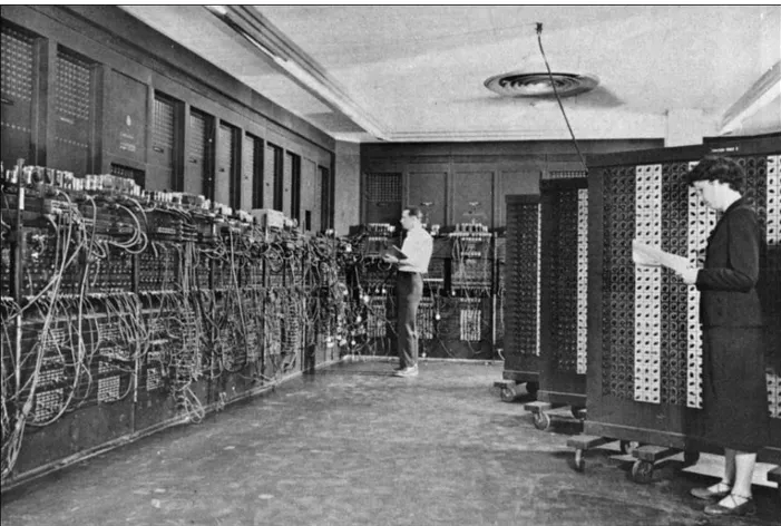
ENIAC
During World War II, the U. S. Navy had battleships with guns that could shoot 2700-pound projectiles 24 miles. At that range, a projectile spent almost 90 seconds in flight. In addition to the guns' elevation, angle of amplitude, and initial speed of propulsion, those trajectories were also affected by the motion of the ship, the weather conditions, and even the motion of the earth's rotation. Accurate calculations of those trajectories posed great problems.
To solve these computational problems, the U. S. Army contracted an engineering team at the University of Pennsylvania to build the Electronic Numerical Integrator and Computer (ENIAC), the first complete
electronic programmable digital computer. Although not completed until after the war was over, it was a huge success.
It was also enormous, occupying a large room and requiring a staff of engineers and programmers to operate. The input and output data for the computer were recorded on Hollerith cards. These could be read
automatically by other machines that could then print their contents.
VisiCalc
In 1979, Harvard student Dan Bricklin was watching his professor correct entries in a table of finance data on a chalkboard. After correcting a mistake in one entry, the professor proceeded to correct the corresponding marginal entries. Bricklin realized that such tedious work could be done much more easily and accurately on his new Apple II microcomputer. This resulted in his invention of VisiCalc, the first spreadsheet computer program for
microcomputers. Many agree that that innovation transformed the
microcomputer from a hobbyist's game platform to a serious business tool.
Data, information, and knowledge
The 1854 cholera epidemic case is a good example for understanding the differences between data, information, and knowledge. The data that Dr. Snow used, the locations of cholera outbreaks and water pumps, was already available. But the connection between them had not yet been discovered. By plotting both datasets on the same city map, he was able to determine that the pump at Broad street and Cambridge street was the source of the
Why Java?
Java is, as it has been for over a decade, the most popular programming language in the world. And its popularity is growing. There are several good reasons for this:
Java runs the same way on all computers
It supports the object-oriented programming (OOP) paradigm
It interfaces easily with other languages, including the database query language SQL
Its Javadoc documentation is easy to access and use
Most open-source software is written in Java, including that which is used for data analysis
Python may be easier to learn, R may be simpler to run, JavaScript may be easier for developing websites, and C/C++ may be faster, but for general purpose programming, Java can't be beat.
Java was developed in 1995 by a team led by James Gosling at Sun
Microsystems. In 2010, the Oracle Corporation bought Sun for $7.4 B and has supported Java since then. The current version is Java 8, released in 2014. But by the time you buy this book, Java 9 should be available; it is scheduled to be released in late 2017.
As the title of this book suggests, we will be using Java in all our examples.
Note
Java Integrated Development
Environments
To simplify Java software development, many programmers use an
Integrated Development Environment (IDE). There are several good, free Java IDEs available for download. Among them are:
NetBeans Eclipse JDeveloper JCreator IntelliJ IDEA
These are quite similar in how they work, so once you have used one, it's easy to switch to another.
Although all the Java examples in this book can be run at the command line, we will instead show them running on NetBeans. This has several
advantages, including:
Code listings include line numbers
Standard indentation rules are followed automatically Code syntax coloring
Listing 1 Hello World program
When you run this program in NetBeans, you will see some of its syntax coloring: gray for comments, blue for reserved words, green for objects, and orange for strings.
In most cases, to save space, we will omit the header comments and the
package designation from the listing displays, showing only the program, like this:
Listing 2 Hello World program abbreviated
Or, sometimes just we'll show the main() method, like this:
Listing 3 Hello World program abbreviated further
Nevertheless, all the complete source code files are available for download at the Packt Publishing website.
Figure 6 Output from the Hello World program
Note
Summary
The first part of this chapter described some important historical events that have led to the development of data analysis: ancient commercial record keeping, royal compilations of land and property, and accurate mathematical models in astronomy, physics, and navigation. It was this activity that led Babbage to invent the computer. Data analysis was borne from necessity in the advance of civilization, from the identification of the source of cholera, to the management of economic data, and the modern processing of massive datasets.
This chapter also briefly explained our choice of the Java programming
Chapter 2. Data Preprocessing
Data types
Data is categorized into types. A data type identifies not only the form of the data but also what kind of operations can be performed upon it. For example, arithmetic operations can be performed on numerical data, but not on text data.
A data type can also determine how much computer storage space an item requires. For example, a decimal value like 3.14 would normally be stored in a 32-bit (four bytes) slot, while a web address such as https://google.com
might occupy 160 bits.
Here is a categorization of the main data types that we will be working with in this book. The corresponding Java types are shown in parentheses:
Variables
In computer science, we think of a variable as a storage location that holds a data value. In Java, a variable is introduced by declaring it to have a specific type. For example, consider the following statement:
String lastName;
It declares the variable lastName to have type String.
We can also initialize a variable with an explicit value when it is declared, like this:
double temperature = 98.6;
Here, we would think of a storage location named temperature that contains
the value 98.6 and has type double.
Structured variables can also be declared and initialized in the same statement:
int[] a = {88, 11, 44, 77, 22};
This declares the variable a to have type int[] (array of ints) and contain
Data points and datasets
In data analysis, it is convenient to think of the data as points of information. For example, in a collection of biographical data, each data point would contain information about one person. Consider the following data point:
("Adams", "John", "M", 26, 704601929)
It could represent a 26-year-old male named John Adams with ID number 704601929.
We call the individual data values in a data point fields (or attributes). Each of these values has its own type. The preceding example has five fields: three text and two numeric.
The sequence of data types for the fields of a data point is called its type signature. The type signature for the preceding example is (text, text, text, numeric, numeric). In Java, that type signature would be (String, String, String, int, int).
Null values
There is one special data value whose type is unspecified, and therefore may take the role of any type. That is the null value. It usually means unknown. So, for example, the preceding dataset described could contain the data point
("White", null, "F", 39, 440163867), which would represent a 39
-year-old female with last name White and ID number 440163867 but whose first
Relational database tables
In a relational database, we think of each dataset as a table, with each data point being a row in the table. The dataset's signature defines the columns of the table.
Here is an example of a relational database table. It has four rows and five columns, representing a dataset of four data points with five fields:
Last name First name Sex Age ID
Adams John M 26 704601929
White null F 39 440163867
Jones Paul M 49 602588410
Adams null F 30 120096334
Note
There are two null fields in this table.
Key fields
A dataset may specify that all values of a designated field be unique. Such a field is called a key field for the dataset. In the preceding example, the ID number field could serve as a key field.
When specifying a key field for a dataset (or a database table), the designer must anticipate what kind of data the dataset might hold. For example, the First name field in the preceding table would be a bad choice for a key field, because many people have the same first name.
Key values are used for searching. For example, if we want to know how old Paul Jones is, we would first find the data point (that is, row) whose ID is 602588410 and then check the age value for that point.
A dataset may designate a subset of fields, instead of a single field, as its key. For example, in a dataset of geographical data, we might designate the
Key-value pairs
A dataset which has specified a subset of fields (or a single field) as the key is often thought of as a set of key-value pairs (KVP). From this point of view, each data point has two parts: its key and its value for that key. (The term attribute-value pairs is also used.)
In the preceding example, the key is ID and the value is Last name, First name, Sex, Age.
In the previously mentioned geographical dataset, the key could be
Longitude, Latitude and the value could be Altitude, Average Temperature, Average, and Precipitation.
Hash tables
A dataset of key-value pairs is usually implemented as a hash table. It is a data structure in which the key acts like an index into the set, much like page numbers in a book or line numbers in a table. This direct access is much
faster than sequential access, which is like searching through a book page-by-page for a certain word or phrase.
In Java, we usually use the java.util.HashMap<Key,Value> class to
implement a key-value pair dataset. The type parameters Key and Value are
specified classes. (There is also an older HashTable class, but it is considered
obsolete.)
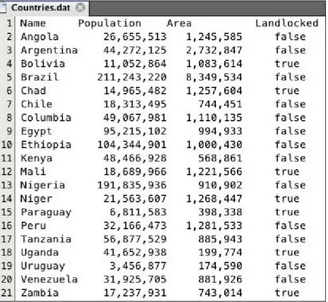
Here is a data file of seven South American countries:
Figure 2-1 Countries data file
Listing 2-1 HashMap example for Countries data
The Countries.dat file is in the data folder. Line 15 instantiates a java.io.File object named dataFile to represent the file. Line 16
instantiates a java.util.HashMap object named dataset. It is structured to
have String type for its key and Integer type for its value. Inside the try
block, we instantiate a Scanner object to read the file. Each data point is
loaded at line 22, using the put() method of the HashMap class.
After the dataset has been loaded, we print its size at line 27 and then print the value for Peru at line 28. (The format code %,d prints the integer value
with commas.)
Here is the program's output:
Notice, in the preceding example, how the get() method implements the
input-output nature of the hash table's key-value structure. At line 28, the input is the name Peru and the resulting output is its population 29,907,003.
It is easy to change the value of a specified key in a hash table. Here is the same HashMap example with these three more lines of code added:
Listing 2-2 HashMap example revised
Line 29 changes the value for Peru to be 31,000,000.
Here's the output from this revised program:
Figure 2-3 Output from revised HashMap program
Notice that the size of the hash table remains the same. The put() method
File formats
The Countries.dat data file in the preceding example is a flat file—an
ordinary text file with no special structure or formatting. It is the simplest kind of data file.
Another simple, common format for data files is the comma separated values (CSV) file. It is also a text file, but uses commas instead of blanks to separate the data values. Here is the same data as before, in CSV format:
Figure 2-4 A CSV data file
Note
In this example, we have added a header line that identifies the columns by name: Country and Population.
For Java to process this correctly, we must tell the Scanner object to use the
comma as a delimiter. This is done at line 18, right after the input object is
Listing 2-3 A program for reading CSV data
The regular expression ,|\\s means comma or any white space. The Java
symbol for white space (blanks, tabs, newline, and so on.) is denoted by '\s'.
When used in a string, the backslash character itself must be escaped with another preceding backslash, like this: \\s. The pipe character | means "or"
in regular expressions.
Figure 2-5 Output from the CSV program
The format code %-10s means to print the string in a 10-column field,
left-justified. The format code %,12d means to print the decimal integer in a
Microsoft Excel data
The best way to read from and write to Microsoft Excel data files is to use the POI open source API library from the Apache Software Foundation. You can download the library here: https://poi.apache.org/download.html. Choose the current poi-bin zip file.
This section shows two Java programs for copying data back and forth between a Map data structure and an Excel workbook file. Instead of a
HashMap, we use a TreeMap, just to show how the latter keeps the data points
in order by their key values.
The first program is named FromMapToExcel.java. Here is its main()
method:
Listing 2-4 The FromMapToExcel program
The load() method at line 23 loads the data from the Countries data file
shown in Figure 2-1 into the map. The print() method at line 24 prints the
contents of the map. The storeXL() method at line 25 creates the Excel
workbook as Countries.xls in our data folder, creates a worksheet named
countries in that workbook, and then stores the map data into that worksheet.
The resulting Excel workbook and worksheet are shown in Figure 2-6.
The code for the load() method is the same as that in Lines 15-26 of Listing
2-1, without line 16.
Here is the code for the print() method:
Listing 2-5 The print() method of the FromMapToExcel program
Figure 2-6 Excel workbook created by FromMapToExcel program
for each of these, we get the corresponding population at line 47 and print them together at line 48.
Here is the code for the storeXL() method:
Listing 2-6 The storeXL() method of the FromMapToExcel program
Lines 60-63 instantiate the out, workbook, worksheet, and countries
objects. Then each iteration of the for loop loads one row into the worksheet
object. That code is rather self-evident.
Listing 2-7 The FromExcelToMap program
It simply calls this loadXL() method and then prints the resulting map:
Listing 2-8 The loadXL() method of the FromExcelToMap program
pair into the map at line 44.
Note
The code at lines 34-35 instantiates HSSFWorkbook and HSSFSheet objects.
This and the code at lines 38-39 require the import of three classes from the external package org.apache.poi.hssf.usermodel; specifically, these three
import statements:
import org.apache.poi.hssf.usermodel.HSSFRow; import org.apache.poi.hssf.usermodel.HSSFSheet; import org.apache.poi.hssf.usermodel.HSSFWorkbook;
The Java archive can be downloaded from
XML and JSON data
Excel is a good visual environment for editing data. But, as the preceding examples suggest, it's not so good for processing structured data, especially when that data is transmitted automatically, as with web servers.
As an object-oriented language, Java works well with structured data, such as lists, tables, and graphs. But, as a programming language, Java is not meant to store data internally. That's what files, spreadsheets, and databases are for.
The notion of a standardized file format for machine-readable, structured data goes back to the 1960s. The idea was to nest the data in blocks, each of which would be marked up by identifying it with opening and closing tags. The tags would essentially define the grammar for that structure.
This was how the Generalized Markup Language (GML), and then the
Standard Generalized Markup Language (SGML), were developed at IBM. SGML was widely used by the military, aerospace, industrial
publishing, and technical reference industries.
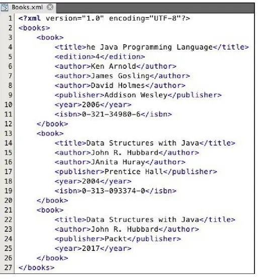
Figure 2-7 An XML data file
This shows three <book> objects, each with a different number of fields. Note
that each field begins with an opening tab and ends with a matching closing tag. For example, the field <year>2017</year> has opening tag <year> and
closing tag </year>.
XML has been very popular as a data transmission protocol because it is simple, flexible, and easy to process.
easy management with Java (and JavaScript) programs. Although the J in JSON stands for JavaScript, JSON can be used with any programming language.
There are two popular Java API libraries for JSON: javax.jason and
org.json. Also, Google has a GSON version in com.google.gson. We will
use the Official Java EE version, javax.jason.
JSON is a data-exchange format—a grammar for text files meant to convey data between automated information systems. Like XML, it is used the way commas are used in CSV files. But, unlike CSV files, JSON works very well with structured data.
In JSON files, all data is presented in name-value pairs, like this:
"firstName" : "John" "age" : 54
"likesIceCream": true
These pairs are then nested, to form structured data, the same as in XML.
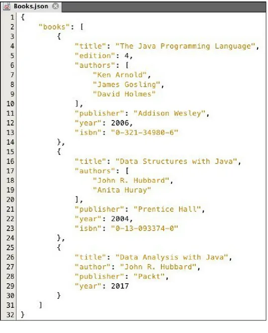
Figure 2-8 A JSON data file
The root object is a name-value pair with books for its name. The value for
that JSON object is a JSON array with three elements, each a JSON object representing a book. Notice that the structure of each of those objects is slightly different. For example, the first two have an authors field, which is
another JSON array, while the third has a scalar author field instead. Also,
Each pair of braces {} defines a JSON object. The outer-most pair of braces
define the JSON file itself. Each JSON object then is a pair of braces, between which are a string, a colon, and a JSON value, which may be a JSON data value, a JSON array, or another JSON object. A JSON array is a pair of brackets [], between which is a sequence of JSON objects or JSON arrays. Finally, a JSON data value is either a string, a number, a JSON object, a JSON array, True, False, or null. As usual, null means unknown.
JSON can be used in HTML pages by including this in the <head> section: < script src =" js/ libs/ json2. js" > </ script >
If you know the structure of your JSON file in advance, then you can read it with a JsonReader object, as shown in Listing 2-10. Otherwise, use a
JsonParser object, as shown in Listing 2-11.
A parser is an object that can read tokens in an input stream and identify their types. For example, in the JSON file shown in Figure 2-7, the first three tokens are {, books, and [. Their types are START_OBJECT, KEY_NAME, and START_ARRAY. This can be seen from the output in Listing 2-9. Note that the
Listing 2-9 Identifying JSON event types
By identifying the tokens this way, we can decide what to do with them. If it's a START_OBJECT, then the next token must be a KEY_NAME. If it's a KEY_NAME,
then the next token must be either a key value, a START_OBJECT or a
START_ARRAY. And if that's a START_ARRAY, then the next token must be either
This is called parsing. The objective is two-fold: extract both the key values (the actual data) and the overall data structure of the dataset.
Listing 2-10 Parsing JSON files
Listing 2-11 A getMap() method for parsing JSON files
Listing 2-12 A getList() method for parsing JSON files
Note
The actual data, both names and values, are obtained from the file by the methods parser.getString() and parser.getInt().
Here is unformatted output from the program, just for testing purposes:
{books=[{year=2004, isbn=0-13-093374-0, publisher=Prentice Hall, title=Data Structures with Java, authors=[John R. Hubbard, Anita Huray]}, {year=2006, isbn=0-321-34980-6, edition=4,
publisher=Addison Wesley, title=The Java Programming Language, authors=[Ken Arnold, James Gosling, David Holmes]}, {year=2017, author=John R. Hubbard, publisher=Packt, title=Data Analysis with Java}]}
The default way that Java prints key-value pairs is, for example, year=2004,
where year is the key and 2004 is the value.
To run Java programs like this, you can download the file javax.json-1.0.4.jar from:
https://mvnrepository.com/artifact/org.glassfish/javax.json/1.0.4. Click on Download (BUNDLE).
See Appendix for instructions on how to install this archive in NetBeans.
Copy the downloaded jar file (currently json-lib-2.4-jdk15.jar) into a
convenient folder (for example, Library/Java/Extensions/ on a Mac). If
Generating test datasets
Generating numerical test data is easy with Java. It boils down to using a
java.util.Random object to generate random numbers.
Listing 2-13 Generating random numeric data
Metadata
Metadata is data about data. For example, the preceding generated file could be described as eight lines of comma-separated decimal numbers, five per line. That's metadata. It's the kind of information you would need, for example, to write a program to read that file.
That example is quite simple: the data is unstructured and the values are all the same type. Metadata about structured data must also describe that
structure.
The metadata of a dataset may be included in the same file as the data itself. The preceding example could be modified with a header line like this:
Figure 2-10 Test data file fragment with metadata in header
Note
When reading a data file in Java, you can scan past header lines by using the
Data cleaning
Data cleaning, also called data cleansing or data scrubbing, is the process of finding and then either correcting or deleting corrupted data values from a dataset. The source of the corrupt data is often careless data entry or
transcription.
Various kinds of software tools are available to assist in the cleaning process. For example, Microsoft Excel includes a CLEAN() function for removing
nonprintable characters from a text file. Most statistical systems, such as R and SAS, include a variety of more general cleaning functions.
Spellcheckers provide one kind of data cleaning that most writers have used, but they won't help against errors like from for form and there for their.
Statistical outliers are also rather easy to spot, for example, in our Excel
Countries table if the population of Brazil appeared as 2.10 instead of 2.01E+08.
Programmatic constraints can help prevent the entry of erroneous data. For example, certain variables can be required to have only values from a
specified set, such as the ISO standard two-letter abbreviations for countries (CN for China, FR for France, and so on). Similarly, text data that is expected to fit pre-determined formats, such as phone numbers and email addresses, can be checked automatically during input.
An essential factor in the data cleaning process is to avoid conflicts of interest. If a researcher is collecting data to support a preconceived theory, any replacement of raw data should be done only in the most transparent and justifiable ways. For example, in testing a new drug, a pharmaceutical
Data scaling
Data scaling is performed on numeric data to render it more meaningful. It is also called data normalization. It amounts to applying a mathematical
function to all the values in one field of the dataset.
The data for Moore's Law provides a good example. Figure 2-11 shows a few dozen data points plotted. They show the number of transistors used in
microprocessors at various dates from 1971 to 2011. The transistor count ranges from 2,300 to 2,600,000,000. That data could not be shown if a linear scale were used for the transistor count field, because most of the points would pile on top of each other at the lower end of the scale. The fact is, of course, that the number of transistors has increased exponentially, not
Figure 2-11 Moore's law
Data filtering
Filtering usually refers to the selection of a subset of a dataset. The selection would be made based upon some condition(s) on its data fields. For example, in a Countries dataset, we might want to select those landlocked countries
whose land area exceeds 1,000,000 sq. km.
For example, consider the Countries dataset shown in Figure 2-12:
Listing 2-14 A class for data about Countries
For efficient processing, we first define the Countries class shown in Listing
2-14. The constructor at lines 20-27 read the four fields for the new Country
object from the next line of the file being scanned by the specified Scanner
object. The overridden toString() method at lines 29-33 returns a String
object formatted like each line from the input file.
Listing 2-15 Program to filter input data
The readDataset() method at lines 28-41 uses the custom constructor at line
34 to read all the data from the specified file into a HashSet object, which is
named dataset at line 19. The actual filtering is done at line 21. That loop
Figure 2-13 Filtered data
In Microsoft Excel, you can filter data by selecting Data | Filter or Data |
Advanced | Advanced Filter.
Sorting
Sometimes it is useful to sort or re-sort tabular data that is otherwise ready for processing. For example, the Countries.dat file in Figure 2-1 is already
sorted on its name field. Suppose that you want to sort the data on the population field instead.
One way to do that in Java is to use a TreeMap (instead of a HashMap), as
shown in Listing 2-16. The dataset object, instantiated at line 17, specifies Integer for the key type and String for the value type in the map. That is
Listing 2-16 Re-sorting data by different fields
The TreeMap data structure keeps the data sorted according to the ordering of
its key field. Thus, when it is printed at line 29, the output is in increasing order of population.
A more general approach would be to define a DataPoint class that
implements the java.util.Comparable interface, comparing the objects by
their values in the column to be sorted. Then the complete dataset could be loaded into an ArrayList and sorted simply by applying the sort() method
in the Collections class, as Collections.sort(list).
In Microsoft Excel, you can sort a column of data by selecting Data | Sort
Merging
Another preprocessing task is merging several sorted files into a single sorted file. Listing 2-18 shows a Java program that implements this task. It is run on the two countries files shown in Figure 2-12 and Figure 2-13. Notice that they are sorted by population:
Figure 2-12 African countries
Figure 2-13 South American countries
Listing 2-17 Country class
By implementing the java.util.Comparable interface (at line 10), Country
objects can be compared. The compareTo() method (at lines 34-38) will
return a negative integer if the population of the implicit argument (this) is
less than the population of the explicit argument. This allows us to order the
The isNull() method at lines 30-32 is used only to determine when the end
of the input file has been reached.
Listing 2-18 Program to merge two sorted files
The program in Listing 2-15 compares a Country object from each of the two
output file at line 27 or line 30. When the scanning of one of the two files has finished, one of the Country objects will have null fields, thus stopping the while loop at line 24. Then one of the two remaining while loops will finish
scanning the other file.
Figure 2-14 Merged files
Note
This program could generate a very large number of unused Country objects.
For example, if one file contains a million records and the other file has a record whose population field is maximal, then a million useless (null)
Hashing
Hashing is the process of assigning identification numbers to data objects. The term hash is used to suggest a random scrambling of the numbers, like the common dish of leftover meat, potatoes, onions, and spices.
A good hash function has these two properties:
Uniqueness: No two distinct objects have the same hash code
Randomness: The hash codes seem to be uniformly distributed
Java automatically assigns a hash code to each object that is instantiated. This is yet another good reason to use Java for data analysis. The hash code of an object, obj, is given by obj.hashCode(). For example, in the merging
program in Listing 2-15, add this at line 24:
System.out.println(country1.hashCode());
You will get 685,325,104 for the hash code of the Paraguay object.
Java computes the hash codes for its objects from the hash codes of the
object's contents. For example, the hash code for the string AB is 2081, which
is 31*65 + 66—that is, 31 times the hash code for A plus the hash code for B.
(Those are the Unicode values for the characters A and B.)
Summary
This chapter discussed various organizational processes used to prepare data for analysis. When used in computer programs, each data value is assigned a data type, which characterizes the data and defines the kind of operations that can be performed upon it.
When stored in a relational database, data is organized into tables, in which each row corresponds to one data point, and where all the data in each
column corresponds to a single field of a specified type. The key field(s) has unique values, which allows indexed searching.
A similar viewpoint is the organization of data into key-value pairs. As in relational database tables, the key fields must be unique. A hash table implements the key-value paradigm with a hash function that determines where the key's associated data is stored.
Data files are formatted according to their file type's specifications. The comma-separated value type (CSV) is one of the most common. Common structured data file types include XML and JSON.
The information that describes the structure of the data is called its metadata. That information is required for the automatic processing of the data.
Chapter 3. Data Visualization
As the name suggests, this chapter describes the various methods commonly used to display data visually. A picture is worth a thousand words and a good graphical display is often the best way to convey the main ideas hidden in the numbers. Dr. Snow's Cholera Map (Figure 1-3) is a classic example.
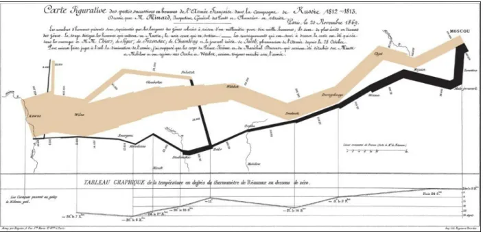
Here is another famous example, also from the nineteenth century:
Figure 3-1. Minard's map of Napoleon's Russian campaign
Tables and graphs
Most datasets are still maintained in tabular form, as in Figure 2-12, but tables with thousands of rows and many columns are far more common than that simple example. Even when many of the data fields are text or Boolean, a graphical summary can be much easier to comprehend.
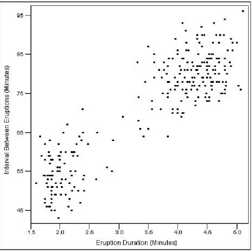
Scatter plots
A scatter plot, also called a scatter chart, is simply a plot of a dataset whose signature is two numeric values. If we label the two fields x and y, then the graph is simply a two-dimensional plot of those (x, y) points.
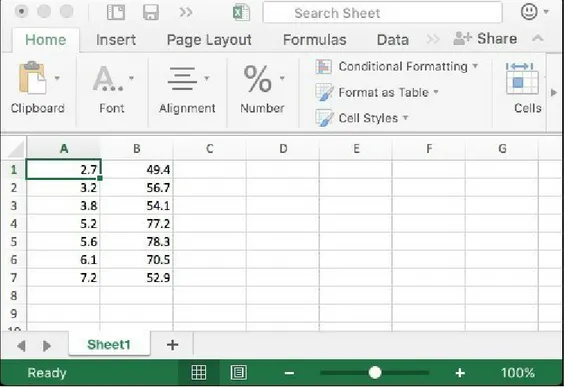
Scatter plots are easy to do in Excel. Just enter the numeric data in two
columns and then select Insert | All Charts | X Y (Scatter). Here is a simple example:
Figure 3-2. Excel data
Figure 3-3. Scatter plot
The scales on either axis need not be linear. The microprocessor example in Figure 2-11 is a scatter plot using a logarithmic scale on the vertical axis.
Line graphs
A line graph is like a scatter plot with these two differences:
The values in the first column are unique and in increasing order Adjacent points are connected by line segments
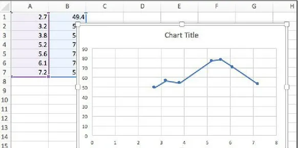
To create a line graph in Excel, click on the Insert tab and select
Recommended Charts; then click on the option: Scatter with Straight Lines and Markers. Figure 3-5 shows the result for the previous seven-point test dataset.
Figure 3-5. Excel line graph
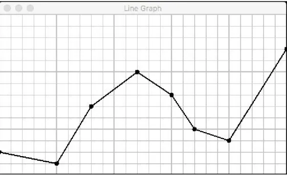
The code for generating a line graph in Java is like that for a scatter plot. Use the fillOval() method of the Graphics2D class to draw the points and then
Bar charts
A bar chart is another common graphical method used to summarize small numeric datasets. It shows a separate bar (a colored rectangle) for each numeric data value.
To generate a bar chart in Java, use the fillRect() method of the
Graphics2D class to draw the bars. Figure 3-7 shows a bar chart produced by
a Java program.
Figure 3-7. Precipitation in Knoxville TN
Bar charts are also easy to generate in Excel:
numeric values.
2. On the Insert tab, click on Recommended Charts, and then either
Clustered Column or Clustered Bar.
The Excel bar chart in Figure 3-8 shows a bar chart for the population column of our AfricanCountries dataset:
Histograms
A histogram is like a bar chart, except that the numeric data represent frequencies and so are usually actual numerical counts or percentages. Histograms are the preferred graphic for displaying polling results.
If your numbers add up to 100%, you can create a histogram in Excel by using a vertical bar chart, as in Figure 3-9.
Excel also has a plug-in, named Data Analysis, that can create histograms, but it requires numeric values for the category labels (called bins).
Time series
A time series is a dataset in which the first field (the independent variable) is time. In terms of data structures, we can think of it as a map—a set of key-value pairs, where the key is time and the key-value represents an event that occurred at that time. Usually, the main idea is of a sequence of snapshots of some object changing with time.
Some of the earliest datasets were time series. Figure 3-10 shows a page of Galileo's 1610 notebook, where he recorded his observations of the moons of Jupiter. This is time series data: the time is written on the left, and the
Figure 3-10. Galileo's notes
More modern examples of time series include biometric, weather, seismologic, and market data.
Most time series data are accumulated by automatic processes. Consequently, those datasets tend to be very large, qualifying as big data. This topic is
explored in Chapter 11, Big Data Analysis with Java.
Digital audio and video files may also be regarded as time series datasets. Each sampling in the audio file or frame in the video file is the data value for an instant in time. But in these cases, the times are not part of the data
Java implementation
Listing 3-1 shows a test driver for a TimeSeries class. The class is
parameterized, the parameter being the object type of the event that is moving through time. In this program, that type is String.
An array of six strings is defined at line 11. These will be the events to be loaded into the series object that is instantiated at line 14. The loading is
done by the load(), defined at lines 27-31 and invoked at line 15.
Listing 3-1. Test program for TimeSeries class
The contents of the series are loaded at line 15. Then at lines 17-21, the six key-value pairs are printed. Finally, at lines 23-24, we use the direct access capability of the ArrayList class to examine the series entry at index 3 (the
Figure 3-11. Output from the TimeSeriesTester program
Notice that the list's element type is TimeSeries.Entry. That is a static
nested class, defined inside the TimeSeries class, whose instances represent
the key-value pairs.
Listing 3-2. A TimeSeries class
The two folded code blocks at lines 43 and 61 are shown in Listing 3-3 and Listing 3-4.
Line 15 shows that the time series data is stored as key-value pairs in a
TreeMap object, with Long for the key type and T as the value type. The keys
used String for the value type T.
The add() method puts the specified time and event pair into the backing
map at line 18, and then pauses for one microsecond at line 20 to avoid coincident clock reads. The call to sleep() throws an
InterruptedException, so we have to enclose it in a try-catch block.
The get() method returns the event obtained from the corresponding map.get() call at line 27.
The getList() method returns an ArrayList of all the key-value pairs in the
series. This allows external direct access by index number to each pair, as we did at line 23 in Listing 3-1. It uses a for each loop, backed by an Iterator
object, to traverse the series (see Listing 3-3). The objects in the returned list have type TimeSeries.Entry, the nested class as shown in Listing 3-4.
Listing 3-3. The iterator() method in the TimeSeries class
The TimeSeries class implements Iterable<TimeSeries.Entry> (Listing
Listing 3-3. It works by using the corresponding iterator defined on the backing map's key set (line 45).
Listing 3-4 shows the Entry class, nested inside the TimeSeries class. Its
instances represent the key-value pairs that are stored in the time series.
Listing 3-4. The nested entry class
Note
This TimeSeries class is only a demo. A production version would also
implement Serializable, with store() and read() methods for binary
Moving average
A moving average (also called a running average) for a numeric time series is another time series whose values are averages of progressive sections of values from the original series. It is a smoothing mechanism to provide a more general view of the trends of the original series.
For example, the three-element moving average of the series (20, 25, 21, 26, 28, 27, 29, 31) is the series (22, 24, 25, 27, 28, 29). This is because 22 is the average of (20, 25, 21), 24 is the average of (25, 21, 26), 25 is the average of (21, 26, 28), and so on. Notice that the moving average series is smoother than the original, and yet still shows the same general trend. Also note that the moving average series has six elements, while the original series had eight. In general, the length of the moving average series will be n – m + 1, where n is the length of the original series and m is the length of the segments being averaged; in this case, 8 – 3 + 1 = 6.
Listing 3-5 shows a test program for the MovingAverage class shown in
Listing 3-5. Test program for the MovingAverage class
Some of the output for this program is shown in the following screenshot. The first line shows the first four elements of the given time series. The second line shows the first four elements of the moving average ma3 that
averaged segments of length 3. The third line shows all four elements of the moving average ma5 that averaged segments of length 5.
Figure 3-12. Output from MovingAverageTester
Listing 3-6. A MovingAverage class
At line 1, the class extends TimeSeries<Double>. This means
MovingAverage objects are specialized TimeSeries objects whose entries
store numeric values of type double. (Remember that Double is just the
wrapper class for double.) That restriction allows us to compute their
The constructor (lines 14-35) does all the work. It first checks (at line 17) that the segment length is less than that of the entire given series. In our test
program, we used segment lengths 3 and 5 on a given series of length 8. In practice, the length of the given series would likely be in the thousands. (Think of the daily Dow Jones Industrial Average.)
The tmp[] array defined at line 21 is used to hold one segment at a time as it
progresses through the given series. The loop at lines 25-27 loads the first segment and computes the sum of those elements. Their average is then
inserted as an entry into this MovingAverage series at line 28. That would be
the pair (1492170948413, 24.0) in the preceding output from the ma5 series.
The while loop at lines 30-34 computes and inserts the remaining averages.
On each iteration, the sum is updated (at line 31) by subtracting the oldest tmp[] element and then (at line 32) replacing it with the next series value and
adding it to the sum.
The nextValue() method at lines 39-42 is just a utility method to extract the
numeric (double) value from the current element located by the specified
iterator. It is used at lines 26 and 32.
It is easy to compute a moving average in Microsoft Excel. Start by entering the time series in two rows, replacing the time values with simple counting numbers (1, 2, …) like this:
This is the same data that we used previously, in Listing 3-5.
Now select Tools | Data Analysis | Moving Average to bring up the Moving Average dialog box:
Figure 3-14. Excel's Moving Average dialog
Enter the Input Range (A2:A8), the Interval (3), and the Output Range
Figure 3-15. Excel Moving Average
These are the same results we got in Figure 3-12.
Figure 3-16 shows the results after computing moving averages with interval 3 and interval 5. The results are plotted as follows:
Data ranking
Another common way to present small datasets is to rank the data, assigning ordinal labels (first, second, third, and so on) to the data points. This can
be done by sorting the data on the key field.
Figure 3-17 shows an Excel worksheet with data on students' grade-point averages (GPAs).
Figure 3-17. Excel data
Figure 3-18. Ranking scores in Excel
Here, we have identified cells B1 to B17 as holding the data, with the first cell
being a label. The output is to start in cell D1. The results are shown in the
Figure 3-19. Results from Excel ranking
Frequency distributions
A frequency distribution is a function that gives the number of occurrences of each item of a dataset. It is like a histogram (for example, Figure 3-8). It amounts to counting the number or percentage of occurrences of each possible value.
Figure 3-20 shows the relative frequency of each of the 26 letters in English language text. For example, the letter e is the most frequent, at 13%. This information would be useful if you were producing a word game like