Python for Microcontrollers Getting Started with MicroPython

(1)

(2)

(3)

Copyright © 2017 by McGraw-Hill Education. All rights reserved. Except as permitted under the United States Copyright Act of 1976, no part of this publication may be reproduced or distributed in any form or by any means, or stored in a database or retrieval system, without the prior written permission of the publisher.

ISBN: 978-1-25-964454-2 MHID: 1-25-964454-5.

The material in this eBook also appears in the print version of this title: ISBN: 978-1-25-964453-5, MHID: 1-25-964453-7.

eBook conversion by codeMantra Version 1.0

All trademarks are trademarks of their respective owners. Rather than put a trademark symbol after every occurrence of a trademarked name, we use names in an editorial fashion only, and to the benefit of the trademark owner, with no intention of infringement of the trademark. Where such designations appear in this book, they have been printed with initial caps.

McGraw-Hill Education eBooks are available at special quantity discounts to use as premiums and sales promotions or for use in corporate training programs. To contact a representative, please visit the Contact Us page at www.mhprofessional.com .

Information has been obtained by McGraw-Hill Education from sources believed to be reliable. However, because of the possibility of human or mechanical error by our sources, McGraw-Hill Education, or others, McGraw-Hill Education does not guarantee the accuracy, adequacy, or completeness of any information and is not responsible for any errors or omissions or the results obtained from the use of such information.

TERMS OF USE

This is a copyrighted work and McGraw-Hill Education and its licensors reserve all rights in and to the work. Use of this work is subject to these terms. Except as permitted under the Copyright Act of 1976 and the right to store and retrieve one copy of the work, you may not decompile, disassemble, reverse engineer, reproduce, modify, create derivative works based upon, transmit, distribute,

disseminate, sell, publish or sublicense the work or any part of it without McGraw-Hill Education’s prior consent. You may use the work for your own noncommercial and personal use; any other use of the work is strictly prohibited. Your right to use the work may be terminated if you fail to comply with these terms.

THE WORK IS PROVIDED “AS IS.” McGRAW-HILL EDUCATION AND ITS LICENSORS MAKE NO GUARANTEES OR WARRANTIES AS TO THE ACCURACY, ADEQUACY OR COMPLETENESS OF OR RESULTS TO BE OBTAINED FROM USING THE WORK,

(4)

OR IMPLIED, INCLUDING BUT NOT LIMITED TO IMPLIED WARRANTIES OF

MERCHANTABILITY OR FITNESS FOR A PARTICULAR PURPOSE. McGraw-Hill Education and its licensors do not warrant or guarantee that the functions contained in the work will meet your requirements or that its operation will be uninterrupted or error free. Neither McGraw-Hill Education nor its licensors shall be liable to you or anyone else for any inaccuracy, error or omission,

regardless of cause, in the work or for any damages resulting therefrom. McGraw-Hill Education has no responsibility for the content of any information accessed through the work. Under no

circumstances shall McGraw-Hill Education and/or its licensors be liable for any indirect,

incidental, special, punitive, consequential or similar damages that result from the use of or inability to use the work, even if any of them has been advised of the possibility of such damages. This

(5)

This book is dedicated to my three wonderful grandchildren, Hudson and Holton Norris and Evangeline Kachavos. They are an absolute joy to be with, although I am sure

(6)

About the Author

Donald Norris has a degree in electrical engineering and an MBA specializing in production

management. He is currently teaching undergrad and grad courses in the IT subject area at Southern New Hampshire University. He has also created and taught several robotics courses there. He has over 36 years of teaching experience as an adjunct professor at a variety of colleges and universities.

Mr. Norris retired from civilian government service with the U.S. Navy, where he specialized in acoustics related to nuclear submarines and associated advanced digital signal processing. Since then, he has spent more than 22 years as a professional software developer using C, C#, C++, Python, Node.js, and Java, as well as 5 years as a certified IT security consultant.

Mr. Norris started a consultancy, Norris Embedded Software Solutions (dba NESS LLC), that specializes in developing application solutions using microprocessors and microcontrollers. He likes to think of himself as a perpetual hobbyist and geek, and is always trying out new approaches and out-of-the-box experiments. He is a licensed private pilot, photography buff, amateur radio operator, and avid runner.

(7)

PREFACE

This is the first book written on the MicroPython language. Although several good tutorials are available on the Web, especially at www.micropython.org , I have found that a book format is often an attractive alternative for readers who do not wish to invest the time and energy needed to wade through online tutorials. In addition, and without disparaging online authors, a wellwritten and -organized book often provides readers a good path to understanding a new and innovative technology such as MicroPython.

I have also presented a few projects in this book, which should interest most readers. There is one on a robotic car, another on building a global positioning system (GPS) sentence decoder, two on how to use Pyboard skins, and one on a let ball detector for those readers who play tennis. The theme of all of the projects is to learn how to interface a MicroPython microcontroller with external devices and sensors.

I cover three separate modules that run MicroPython in this book. The first is the Pyboard, which was designed by Dr. Damien George, who is also the creator of the MicroPython language. All of the introductory scripts are run on the Pyboard, as well as all of the book’s projects. The other two

boards discussed are the ESP8266 and the WiPy. These boards run MicroPython, but they also have a built-in wireless radio system, which is lacking in the Pyboard. In fact, the WiPy has four separate wireless radio systems, which makes it quite a chameleon if you need a module that can connect to a variety of wireless protocols. Learn all about it in Chapter 10 .

The reader should expect a great increase in knowledge of and experience with MicroPython if a commitment is made to read all of the introductory material as well as to complete most of the

projects. I personally always learn a great deal while designing and finishing them. Often, things work out just fine, whereas at other times they are fraught with problems. However, that’s what I consider the joy of experimenting. As the renowned Professor Einstein once stated, “Anyone who has never made a mistake has never tried anything new.”

I would caution any experienced Linux developers to at least review the beginning chapters

because MicroPython, although modeled after Python 3, does have a few “gotchas” that one should be aware of before wading too deeply into the MicroPython pool. I have tried to provide many useful hints and techniques throughout the book to assist readers in this MicroPython adventure.

So, without further ado, let the adventure begin.

(13)

ACKNOWLEDGMENTS

I first

thank my lovely wife, Karen, for putting up with all my experiments and enduring all the “discussions” about the book projects.

Thanks go to Michael McCabe for his fine support as my editor and also to Amy Stonebraker for her support as editorial assistant.

In addition, thanks go out to Anju Joshi for her fine work as the project manager.

(14)

1 Introduction

This book

is about the MicroPython language; it includes eight projects using the Pyboard, the ESP8266 or the WiPy board. Projects using one of these boards will be discussed in great detail in later chapters; however, I will be using the Pyboard to introduce the MicroPython language because it comes installed in it and ready to use.

Introduction to MicroPython

MicroPython is a variant of the Python 3 language designed specifically to run on

memory-constrained microcontrollers. It was the idea of Dr. Damien P. George of Cambridge University, who first created an initial version in 2013 along with a Kickstarter campaign to fund the production of the Pyboard, which is a specially designed hardware development board hosting MicroPython as an operating system (OS). Dr. George subsequently presented MicroPython, version 1.0, at a 2014 Python Conference (PyCon). Dr. George also started the website micropython.org to support both the language and the Pyboard. All the latest information regarding the MicroPython language and the Pyboard may be found on this website. There are also several very active user forums hosted on this site, which I found to be very beneficial in answering questions I had on MicroPython and the

Pyboard.

Design Philosophy

At the outset, I would like to disclose my design philosophy regarding the proper use of MicroPython and the Pyboard. You should note that this disclosure only represents my philosophy and not

necessarily Damien George’s approach, although I would suspect that they are not too different. MicroPython as implemented on the Pyboard is designed to quickly and efficiently create control programs for embedded projects. An embedded project can be simply defined as any project that requires the use of a microcontroller to meet project requirements, with or without human

intervention. Typical embedded projects often use sensors and sometimes electromechanical actuators, which are interfaced to the microcontroller. They may have human interface devices

(15)

Embedded projects usually do not require or need general-purpose applications such as a terminal program or a database program. MicroPython does not easily support adding such high-level

applications. You are likely using an inappropriate board if you find that you require these types of applications for your project. A Raspberry Pi or BeagleBone Black would likely be a much better fit for your project, as both support powerful Linux distributions that are easily adapted and configured to meet high-level requirements.

In summary, MicroPython and the Pyboard are best suited for rapid development of embedded applications using a high-level language. Such applications are very efficient when operating and use minimal memory compared with more traditional development approaches.

Exploring MicroPython

Before I start delving into the intricacies and fine details of both Python and MicroPython, I thought I would show both logos. Figure 1-1 shows the logo of the official Python language, which can only be formally associated with Python language implementations recognized and supported by the Python organization at python.org. It is also known informally as the two snakes logo.

Figure 1-1 Official Python logo.

(16)

Figure 1-2 MicroPython logo.

The interesting aspect is that the Python name is not based on the python snake species, but rather springs from Python creator Guido van Rossum’s interest in the U.K. comedic group Monty Python.

In the next section I will present object-oriented (OO) concepts along with a discussion on the Python language describing its main features and its original intent. This will be necessary to understand why MicroPython was created and why it is truly an important addition to the Python community. Feel free to skip the next several sections if you are already quite comfortable with using Python and object-oriented technology and just really want to start using MicroPython.

Object-Oriented Programming and Some Python Basics

Let me first state that this section is not intended to be a tutorial on either OO or Python. There are many fine tutorials freely available on the Web covering both topics, which can provide a much better background than I could possibly provide. My intention is to provide a sufficient background in both object-orientation and key Python concepts to enable you to gain a good understanding of both what makes Python function so well and why you should use it for your microcontroller projects. You should read this material keeping in mind that if some concept is fuzzy or unclear it might behoove you to research it further before continuing with this book. Thankfully, no quizzes or exercises are associated with this section other than one incredibly easy question, which I will discuss shortly.

Object-Oriented Concepts

To begin our exploration of object orientation, let us pretend we have been transported to a virtual environment where objects are the primary life form. We will call this environment Object Land.

Figure 1-3 shows a very abstract view of Object Land where two processes are shown (small and big), each containing multiple objects that are in constant communication with one another to

accomplish the overall process goals. The processes themselves are communicating with each other as needed to accomplish whatever needs to be done.

(17)

A key question arises: What is an object?

The textbook answer typically given is that an object is an instance of a class. Of course, this only further confuses the newcomer to Object Land where he (used only in the generic sense) doesn’t know the definition of a class. OK, so what is the definition of a class and, more important, why should I care?

First, a quick quiz. What does Figure 1-4 represent?

Figure 1-4 Unknown object.

Bus Train Race car Plane

The answer really lies with your life experience. Most people will know it is a race car by its shape and the fact that the driver is wearing a helmet. Others may recognize it by the process of elimination by realizing it is not a bus, train, or plane. We engage in this process continuously—that is, we use models or abstractions to represent real-world things or objects.

Similar activities are present in software design where we use abstractions to represent real-world things. This approach is much more relevant in developing software compared with a much stricter procedural approach. Consider a situation where you at the train station exit having just arrived in New York City. Now you want to go to Radio City Music Hall and take in a show, so you hail a cab. Once in the taxi, do you tell the driver, “Go to the end of the street; take a right; go through two sets of lights; take a left . . .” or do you simply say “Please take me to Radio City Music Hall”? The first approach is procedural, whereas the latter is object oriented. In taking the OO approach, you are relying on that person object (the taxi driver) to be responsible for accepting a message “Please take me to Radio City Music Hall” and know how to accomplish the task. One very nice feature of this approach is that the object may have to change its implementation depending on traffic, street closures, etc., but you as the message sender will not be aware of this change. You have to be aware of all the traffic conditions in New York City if you choose the procedural approach. Not a very appealing situation!

Having established the fact that objects will in fact be useful to accomplish your goals in

(18)

programming (OOP) paradigms. Table 1-1 lists the four bedrock principles that apply to all OOP languages.

Table 1-1 Four Bedrock Object-Oriented Principles

A handy mnemonic to remember these principles is APIE, taken from the beginning letter for each principle.

I decided to use a generic robot as a model to demonstrate how to apply the OO approach. Determining basic robot characteristics and behaviors is normally the first step in creating a class. The class is the data structure used to record these characteristics and behaviors. In formal OO terms, characteristics are known as attributes, and behaviors are methods. Objects are created from classes. As mentioned earlier, an object is simply an instance of a class. How this is done depends on the specific language being used. Many OO languages such as Java, C#, and C++ use the new operator to

create a class instance. In Python, all you need to do is use the assignment operator or = symbol. This process is known as instantiation.

It is often useful to refer to basic definitions in developing class attributes and methods. Many robot definitions are available, but I have created one that fits my understanding and belief of what a robot is, and it is one that I believe you will find useful when trying to create a robot class definition: a robot is a system with sensors, actuators, and a feedback control mechanism . Note that I avoided the use of the words knowledge and intelligence . It is readily apparent that robot can appear

intelligent; however, I want to side-step the whole artificial intelligence discussion for now. In addition, the word actuators implies the action or motion normally associated with robots. Some robots are quite mobile, whereas others are fixed in place, such as a robotic work cell. Additionally, the reference to a feedback control mechanism implies the use of (a) sensor(s) and the ability to react to the data generated by the sensor(s).

The key is to try to encapsulate all the essential attributes and behaviors that are useful in

describing a real-world object in a logical data structure such as a class. I also wish to emphasize that there is really no one correct answer to creating a class. It turns out some descriptions are better than others, and you will find that as you proceed with your design you will often go back and revise your initial class definition. Experience in repeated OO design efforts will improve your initial

efforts, and incorporating design patterns (DPs), which I discuss later, will also help with the design. I have repeatedly told my beginning OO students that creating classes are probably the single hardest task to tackle in the whole OO approach.

Modeling a Robot

(19)

robot, which provides a good template to model other, more specific robot types. Figure 1-5 shows a simple robot inheritance class diagram with a parent class and four child classes. The parent class contains the general attributes and methods common to all the child robot classes. Unified Modeling Language (UML), version 2, standards were followed in constructing Figure 1-5 . UML is the

software development industry’s standard way of displaying graphical models. Knowing how to create useful UML diagrams promotes efficiency and effectiveness in communicating your design ideas to others in the development process.

Figure 1-5 Robot UML class diagram.

The four child classes—namely Wheeled, Tracked, Legged, and Flying—get their names from their primary mode of movement. These four robot subclasses can be instantiated as they have specific implementations for the methods declared, but not implemented, in the parent class.

Inheritance is very useful in promoting software reuse, but it does have its drawbacks. It must be used in a very careful approach to avoid situations where too many unique objects could be created by combining different parent case attributes and/or methods. Interfaces will be discussed later as a more elegant way of creating objects with limited use of inheritance.

(20)

without granting the entities permission. Scope enforces this constraint by setting attributes and

methods as private, public, or protected. Private scope means exactly what its name states: attributes and methods are only available within the encompassing class and consequently all objects

instantiated from that class. Outside entities cannot change, modify, or delete private attributes or methods. A minus sign (–) in front of a UML entry indicates private scope.

Attributes and methods marked as public are available to outside entities. However, attributes themselves are rarely made public because that typically destroys class encapsulation. Public

methods, on the other hand, are the way classes allow messages to be both received and sent by class objects. This approach is termed the public interface, and for the vast majority of situations, is the way classes are created. In some advanced OOP areas there are inner classes that do not require a public interface to achieve the desired functionality. Inner classes will not be required for sensor programming. A plus sign (+) in front of a UML entry indicates public scope.

The final type of scope is protected. This is almost identical to private, except child objects are permitted access to parent attributes and methods declared protected, but no other outside entity is granted permission. Protected scope helps with inheritance class structure implementations, and child objects are always treated as if they are the same type as the parent. From our robot class diagram we can make the statement “A Wheeled or Tracked object is a Robot object.” Inheritance is always the “is a” relationship.

Another key concept to consider is composition, which is a situation where a class contains attributes that are objects instantiated from other classes. Composition allows us to build complex objects, just as real-world things are made up of different components. Consider a car that contains an engine. You can easily imagine a Car class; however, it would be a big mistake to create a child class named Engine. It would fail the commonsense inheritance test of stating “an Engine is a Car,” which is required for true inheritance to exist. However, you can state with confidence, “a Car has an Engine.” Composition is the “has a” relationship. Composition and the closely related aggregation relationship concept are extremely helpful in creating useful and descriptive classes and are needed to successfully implement the interface concept mentioned earlier.

An interface is a specialized class that only contains methods and no attributes. Classes using interfaces can supplement the methods that are declared either within the class or within a parent class if inheritance is used. Interfaces also support inheritance to allow for specialized method implementations that fit specific subclass requirements. An example is really needed to clarify how interfaces are best used.

Some Python Basics

I felt it important to now cover some basic Python concepts before presenting some example code implementing the general OO principles I presented earlier. I will first start by stating that Python is a true OO language, strictly adhering to the APIE bedrock principles shown in Table 1-1 . Sometimes, programmers become confused and misled by Python’s interactive nature; but make no mistake—it is truly an OO language, capable of implementing most, if not all, of the sophisticated implementations that developers can dream up.

I will be using Linux running on a Raspberry Pi 2, Model B, for the sake of simplicity and

(21)

discussion purposes are minimal, and I will point out where they exist. Figure 1-6 shows an

interactive session in which I have input several different operations and assignments to demonstrate some Python actions.

Figure 1-6 Python interactive session.

At first you should note that I started the Python interpreter by simply entering python at the RasPi’s command-line prompt. This brings up the Python interactive prompt >>> along with some introductory words. I next entered a simple addition of two integer numbers, which was immediately executed after I pressed the ENTER (RETURN ) key. Python will always try to execute any properly

entered expression and return the results, if any, to the user.

The next entry shows how to allocate and initialize a variable—in this case, a variable named a, which is set to a value of 6. No return value is shown, nor is there any error message, which means that Python both accepted the variable assignment and its initialization. This simple step actually reveals something quite remarkable about Python, in that it is a strongly typed language and it invokes dynamic allocation. This means that Python dynamically created a variable named a that holds or stores integer (whole) numbers. I could have later on reassigned a value of 6.0 to a, which would have caused Python to change the a variable type from integer to floating point or real, that is, a number containing a decimal point. This action is known as dynamic typing and makes it easy for users to create programs or scripts without much forethought, although there are some inherent problems lurking if you are not careful.

The next few steps in the figure show how two more variables were created: one initialized to a hard value and the other the sum of the two previous variables. I then entered the last variable, c , and pressed ENTER . Its computed value was immediately displayed.

(22)

to a real number, 9.0, and repeat the calculation, and voila: 4.5 was the correct response.

The last calculation of 13 % 6 demonstrates integer remaindering where the % operator returns the

remainder of the expression—in this case, 1. This % operator is also known as the modulo operator,

and I find it quite useful for specific math calculations.

It would be impractical and very inefficient to only have the interactive mode available to Python users. Fortunately, Python allows for prewritten programs or scripts to be executed. These function precisely the same way as if a user entered them directly via the interactive interpreter. However, scripts offer more in that many predefined modules such as classes can be quickly referenced and instantiated, allowing for a fully featured OO development environment. From this point on, I will only be using Python programs to demonstrate the language and all its OO capabilities. Note that you should use any text editor you feel comfortable using as the means to enter the code shown in this book. I will be using the nano editor, which is readily available for installation on the RasPi by entering the following command:

I also believe that nano already comes installed in the latest Raspian Linux distributions. You may also copy and paste the code from this book’s companion website,

www.mhprofessional.com/micropython .

The Robot Class

The following Python code defines my first attempt at modeling a generic robot using the guidelines I discussed earlier. There are only two key behaviors, move and sense, that are common to all the

robot subclasses as defined in the UML model. Child classes that use these behaviors, or methods as I shall call them from now on, also provide specific method implementations suitable for their

respective robot models.

(23)

I will next discuss two of the four child classes shown in Figure 1-5 .

Child Classes

This section will demonstrate how to create WheeledRobot and TrackedRobot child classes. Print line statements will be used, as that is the simplest and most effective way of showing object behavior without using actual hardware.

I will also use two of the methods detailed in the Robot class diagram, as this will be sufficient to illustrate object interaction and behavior. These methods are:

perform_move()

perform_sense()

(24)

In Python, an inheritance relationship is created simply by placing the parent class name in parentheses after the child class name. In this situation, the statement:

creates the inheritance relationship that the Robot class is a parent of the child class WheeledRobot. In many OO languages, there is a special method known as a constructor, which initializes an object’s attributes to known and consistent states prior to use. Python does not use a constructor, per se, but instead uses the __init__ method, which is very similar in functionality to the constructor. In this class definition, the __init__ method associates the appropriate movement and sense functions to the object, which will be moving with wheels and sensing distance using a Ping ultrasonic sensor.

The TrackedRobot class is set up in a similar fashion to the WheeledRobot class and is shown next.

The most important design criteria associated with OO languages, including Python, is the ability to both modify and reuse existing software modules. Doing both of these functions without upsetting or “breaking” the existing code base is the subject of the next section regarding interfaces.

Using Interfaces

(25)

Figure 1-7 Interface UML diagram.

The following is the MoveBehavior class definition code listing. It is quite brief and only exists to serve as a parent for the class interface hierarchy.

The SenseBehavior class definition is almost identical to the MoveBehavior class and will not be shown.

Next, the child class definition associated with movement for a wheeled robot is listed.

(26)

message. In a real-world situation, this class definition could be very complex, involving many

commands and physical interfaces associated with a real wheeled robot. The MoveWithTracks class definition is almost identical to the previous listing, except it contains a slightly different print

message.

The SenseWithPing class definition is shown next.

This code listing follows the same template as the movement behavior child classes, which is a good indication of the simplicity and consistency of this design approach.

The next section ties the Robot class design and the interface design together and presents a test class to prove that the overall project functions as expected.

Integrated Robot Project Design and Test

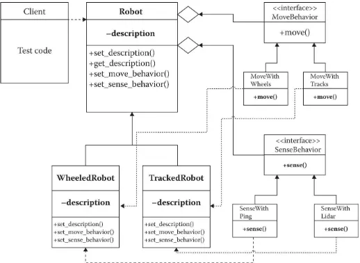
The complete robot project UML diagram with the robot parent and subclasses, as well as the

behavior interface classes, along with the respective subclasses are shown in Figure 1-8 . A test class is also shown in the diagram, which is labeled as a client to conform to typical UML designations.

(27)

Note that the interface subclasses that represent the behavior portion of the project for specific robots are connected to the appropriate Robot subclass blocks using dashed lines. This UML designation indicates that the behavior interface classes help compose part of the class but are not strictly part of the class definition, which is consistent with my earlier discussion regarding

composition.

The test code block, labeled client, is also attached to the Robot class with a dashed line, but this relationship is just to indicate that the client needs to instantiate or create some Robot objects to carry out its intended functions. The test code contains no class definitions and simply calls several public methods made available by the Robot class.

The following is the program listing for test_code.py:

There are obviously a lot of import statements, as this is the way Python assembles or references all the different classes that make up this project. You should also note that I only instantiated two objects in the code, wheeled and tracked, that reference the WheeledRobot and TrackedRobot classes, respectively. Additionally, all the print statements in the code simply make the program output easier to read.

(28)

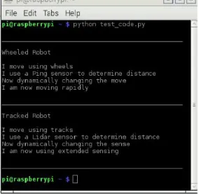
Figure 1-9 Test code output.

The previous discussion was lengthy but necessary to illustrate a good approach to creating code that is understandable and fairly easy to adjust to accommodate changing requirements. Another important principle underpinning this methodology is to:

Favor composition over inheritance.

Using the interfaces with the child implementation classes is a concrete example of applying this principle. The code was made robust by recognizing that movement and sense behaviors will be different for different robot types. So instead of trying to hard-code specific types of behavior in each of the concrete Robot subclasses, I chose to pull that all out and place it in the interfaces. This

apparent recognition of object differences leads to one more principle: Identify what varies and encapsulate it.

Movement and sense vary for each type of robot, so those behaviors were pulled out of the Robot class and delegated to interfaces. Then, appropriate interface implementation subclasses were

created to invoke the specific behavior for that Robot object with that type of behavior. Very simple and somewhat elegant!

I have saved the best for last in this discussion. The approach I have taken with creating this code is an example of the design pattern strategy. Design patterns (DPs) are often introduced into advanced computer science courses; however, I believe if you learn the patterns early on, you will develop good code design practices that will help you in all your future development efforts. DPs in software development have been around since 1995, when the book Design Patterns 1_{was published. DPs are}

not specific solutions to specific problems, but are a methodical approach for creating good solutions given a general type of problem domain. They are based upon years of great software development by masters in this field, “standing on the shoulders of giants,” as the old saying goes.

Dynamic Binding

(29)

These are set_move_behavior(self, mb) and set_sense_behavior(self, sb) . These methods

allow Robot objects to reference both movement and sense behaviors as needed during program execution. This modus operandi is called dynamic or late binding, as compared to establishing fixed references that occur during the compilation stage, which is called static or early binding. Dynamic binding is interesting from the perspective that robots can change their movement and sense behaviors to suit real-time conditions. I have created two more interface implementation classes to illustrate dynamic binding. Don’t get too excited, however, as all they do is output a slightly different console message compared to the original class message. The two new classes created are

StartRapidMoveOnTheFly and StartExtendedSenseOnTheFly. These two new classes are listed next.

(30)

(31)

Figure 1-10 Terminal output with dynamic behavior set.

An additional text message, “Now dynamically changing the move (sense),” is displayed just before the call to perform the move or sense associated with the newly reallocated behavior instance variables move_instance and sense_instance. The messages “I am moving rapidly” and “I am now using extended sensing” come from the new classes I just incorporated into the project. Dynamic binding is also considered polymorphic behavior in that sending exactly the same message invokes different responses from the target objects. In this case, the message (or method call) is

wheeled.perform_move() for the WheeledRobot object and tracked.perform_sense() for the

TrackedRobot object.

On-the-fly or dynamic reconfiguration of robot behavior provides a huge amount of flexibility in coping with real-time situations. Consider the case where a reconnaissance robot has been deployed into a battlefield situation. Sometimes field conditions change, such as the addition of smoke or fog, inhibiting normal robot movement and/or sensing. Reconfiguring the robot to accommodate to the new environment would allow the reconnaissance robot to continue its mission. Installing new behavior to match the mission is easily accomplished with dynamic binding.

It is important to realize that dynamic binding is simply not possible using a strict inheritance structure. The added flexibility that interfaces provide is yet another reason that most developers favor using interfaces over strict inheritance.

This last section concludes my introductory discussions regarding OO, Python basics, and a recommended software design approach. It is now time to start using MicroPython.

Using MicroPython with a Pyboard

(32)

computer using a micro USB cable. I used a version 1.1 Pyboard, which I purchased from Adafruit.com and whose part number is 2390. This Pyboard is shown in Figure 1-11 .

Figure 1-11 Version 1.1 Pyboard.

(33)

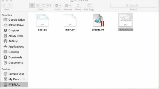
Figure 1-12 Contents of the PYBFLASH drive.

There is a file named README.txt, which you should open, as it contains instructions on how to start a terminal session with the Pyboard according to which OS you are using, that is, Windows, Mac, or Linux. Figure 1-13 shows the contents of this Readme file.

Figure 1-13 Readme file for establishing a terminal session.

(34)

Figure 1-14 MicroPython initial welcome screen.

At this point you are interacting with a “regular” Python session such that you can enter

expressions and see immediate results as previously shown in the chapter. MicroPython behaves identically to ordinary Python at this level. This interactive interpreter mode is also known as REPL, which is short for read-eval-print-loop. It is one of three ways the user can interact with the Pyboard. The other two modes will be discussed in the next chapter where I explain how to use programs with the board. Meanwhile, the REPL mode is by far the easiest and most convenient way to work with the Pyboard.

You should also be aware that there is only about 200 kB of random access memory (RAM) available, and you will rapidly run out of memory if you attempt to deal with objects and/or

expressions that consume substantial memory. However, there is a good option available to help with this constrained memory. That option consists of a micro SD card socket, which you can see is

located next to the micro USB connector in Figure 1-11 . Plugging a 4-GB card into this socket will vastly enhance the amount of memory available to the Python OS and allow you to create basically unlimited sized programs. My strong recommendation is that you only use a relatively high-speed class 10 micro SD card in order to minimize any processing delays that will likely occur when transferring data between the card and the Pyboard.

Bare-Metal Approach

I am concluding this first chapter with a discussion of the bare-metal approach that Dr. George decided to take when creating MicroPython. These points come in large part from his July 17, 2015, podcast “Python on bare metal with MicroPython” on talkpython.fm, episode #17.

It should be made clear at this point that MicroPython is a complete rewrite of Python version 3.4. The main goals in this rewrite were to make this Python version as efficient as possible and to use the least amount of RAM necessary to execute any operation.

(35)

microcontroller installations, such as may be found in the RasPi I used earlier in the chapter. Having such intimate control of machine operations allows the developer to create the most efficient

programs possible, while still programming at a relatively high abstract level with the Python language.

It is also possible to include in-line assembly code into a MicroPython program. You should also be aware that MicroPython has an option to generate assembly code in any one of three formats: bytecode, ARM code, and finally direct machine code. The bytecode format is the default mode for the MicroPython compiler. Every instruction or data entry contained in a Python program is

eventually compiled into bytecode before being executed. Some developers seem to be ignorant of this fact when they state that Python is slow. It is a strictly interpreted language as compared to a strictly compiled language such as C. The truth is that although Python does use a line-by-line

interpreter, it also employs a very fast compiler for bytecode generation. This approach also mirrors how the Java language functions, which is good. CPython, which is based on a C runtime, actually is comparable in terms of speed with MicroPython running on a microcontroller such as the Pyboard. However, this comparison is somewhat faulty and is really like comparing apples to oranges in that you cannot load CPython onto a Pyboard due to memory constraints. Speed comparisons actually can be made on a PC, where it is totally possible to run instances of both MicroPython and CPython. However, the key point to realize here is that MicroPython is no longer running in a bare-metal environment and must operate in compliance with a host OS, which certainly hinders its efficiency. Nonetheless, it still operates quite well.

Dr. George also points out that MicroPython was never meant to replace C, but just to provide developers with an extremely efficient way to program a microcontroller while using the friendly, high-level Python language.

This last section concludes this chapter’s introductory discussions. Much more detailed information on MicroPython starts in the next chapter.

Summary

The chapter began with a brief history of the MicroPython project and its connection to the regular Python language.

A discussion of object-oriented concepts followed as I considered it important that readers understand these principles in order to fully appreciate and properly utilize this language.

The next section addressed how to model a robot using OO techniques. I also briefly discussed some basic Python concepts in order to lay the groundwork for the Python code that followed. This code implemented a robot parent class and several specific robot child classes.

I next introduced the concept of interfaces and explained how they can greatly improve the quality and maintainability of a code project. These interfaces were then incorporated into a comprehensive robot package that included some test code to demonstrate that the code functioned as desired. The test code was then modified slightly to demonstrate how dynamic binding worked.

The next section demonstrated how to boot up MicroPython on a Pyboard using the REPL mode of operation.

(36)

Dr. Damien George.

1_{Erich Gamma, John Vlissides, Ralph Johnson, and Richard Helm,}_{Design Patterns: Elements of Reusable Object-Oriented}_,

(37)

2 Introduction to the Pyboard

This chapter

will focus on how MicroPython is used with the Pyboard. It is not intended to be a reference chapter, but more of personal introduction where I explain the hardware and how the MicroPython software enables the board functions. This approach seems to me a good one in that MicroPython is crafted to be very “close” to the way the hardware functions. However, feel free to go back and reference this material as you progress through the remainder of the book, as you will likely need to refresh yourself on certain topics that may seem cloudy or unclear the first time you encounter them.

Pyboard Hardware

The Pyboard was especially created for MicroPython. It is not a repurposing or porting of an existing microcontroller board. It is also completely open source, with schematics freely available for your own use, whether for personal or commercial use, under the terms of the MIT license. I do urge you to review this license before you attempt to commercialize a product based on the Pyboard design. The license is extremely generous in nature, but you do have to comply with some conditions, especially recognizing the design’s creator.

(38)

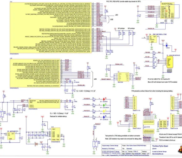
Figure 2-1 Pyboard schematic.

I realize that this figure is probably quite difficult to interpret given the book’s limited dimensions. You download the schematic in a PDF format from the www.micropython.org website. It can be found in the Docs area.

(39)

Table 2-1 Pyboard Integrated Chips and Their Functions

(40)

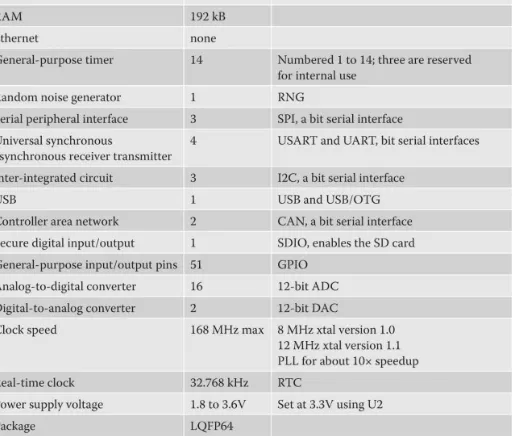
Table 2-2 Key Specifications for the Pyboard STM Micro

A complete PDF datasheet for this STM microcontroller can be downloaded from the STM website at www.st.com . I highly recommend that you download this 201-page PDF, as it contains detailed explanations of all the microcontroller features you will need when creating programs for this chip. Based upon my experience as a professional embedded developer, having a microcontroller datasheet readily available is an invaluable asset for successful program development. There are just too many fine details regarding modern-day microcontrollers, which makes it imperative to read and understand the information contained in the datasheet, which has been prepared by the engineering design team.

At this point, I will digress a bit and discuss some key aspects of generic microcontroller programs, independent of any implementation language such as MicroPython.

(41)

In the late 1970s, an extremely popular 8-bit microcontroller named the 8051 was introduced by Intel. It was quite limited in its capabilities and functionalities as compared with today’s 32-bit

microcontrollers, but later versions are still incorporated into many millions of products and projects. The interesting fact about the 8051 is that there is no host operating system for this chip. Any program executed on an 8051 was required to implement all memory, file, and resource utilities as needed and at the same time keep program sizes to an absolute minimum. Fortunately for most developers, an excellent set of C libraries were available that met most of the project requirements, yet used

precious little of the available ROM memory space. There was essentially only a single program run on the chip, which consisted of an infinite loop that had to be interrupted at times to service events such as data entry or taking a sensor measurement. This process of using interrupts became second nature to not only 8051 developers, but to anyone else using a similarly configured chip. This

situation still holds true in today’s development world where interrupts are still critical for efficient and effective microcontroller operations. The STM micro used on the Pyboard offers a whole array of different interrupts to help create programs that are both efficient and responsive. The MicroPython language offers high-level, direct control over interrupts, which is a unique feature not found in any other object-oriented (OO) language of which I am aware.

The preceding brief discussion was a prelude and justification for this next section, which

discusses interrupts and where I will also create a simple interrupt demonstration using MicroPython.

Interrupts

(42)

Figure 2-2 Interrupt sources and flow diagram.

Hardware

Exceptions and traps

Direct software instructions

Hardware interrupts may be generated by a vast array of devices that need the attention of the processor. Interrupt events might be the immediate availability of sensor data or the sudden increase in a device input voltage level over some preset threshold value. These hardware interrupt requests (IRQs) are directly connected to the STM micro using any one of 16 GPIO lines. The STM micro also has a built-in interrupt/event controller (EXTI) to manage all of these possible IRQs in an orderly fashion.

(43)

Forced or deterministic software interrupts (SWIs) are the last interrupt source category. SWIs are places in a program where an interrupt is forced for a particular reason. It often may be used to

terminate a program at a specific time or after a preset computed value has been reached. An SWI could also be used to jump to an interrupt handler based upon some metric regarding the amount of memory used so that additional memory can be allocated before the program is abnormally terminated through an out-of-memory exception.

Figure 2-2 also shows a generalized diagram of what steps the processor will take when an interrupt is recognized and processed. The first step is always to complete processing the current instruction that was being handled when the interrupt happened. Next the processor state is saved on to a memory stack, which is just a series of preset memory locations where data such as the program counter (pc) is stored. The pc is important, as that contains the memory location for the next

instruction to be executed by the processor. This shows the processor “knows” where to resume its normal processor flow after the interrupt is handled. It simply jumps back to the restored pc location and begins again as if nothing had happened. Of course, other key data registers are also

automatically restored so that the complete processor context is as it was prior to the interrupt. The processor will jump to a preset interrupt handler routine based on the interrupt source and its priority. The STM micro has another built-in controller, named the nested vectored interrupt

controller (NVIC), which handles up to 16 priority levels and up to 82 maskable interrupt channels, plus the 16 interrupt lines of the STM micro. Maskable interrupts are those that can be software disabled while still having some higher-priority nonmaskable interrupts activated. Of course, disabling all interrupts prevents both maskable and nonmaskable interrupts from interrupting the processor. The NVIC knows the address of the interrupt handler to jump to based on the interrupt source and its priority. The term nested in the NVIC name refers to the fact that it allows higher-priority interrupts to interrupt lower-higher-priority ones while keeping track of all the return addresses so that the processor does not fail in processing all these interrupts in a proper sequence.

Hardware interrupts from connected devices on the STM micro can be triggered by a variety of changes occurring on the pin connection. These include

1. Voltage transition from low to high (rising edge trigger) 2. Voltage transition from high to low (trailing edge trigger) 3. Voltage state change from low to high

4. Voltage state change from high to low

There is only a slight timing difference between the edge triggers and state change triggers, where edge triggers are more sensitive to an immediate IRQ, whereas the state change has a small settling time before triggering an IRQ. Select the appropriate type that best matches the timing and interrupt requirements for your project.

My final point in this discussion is to point out that each interrupt handler must be designed to completely satisfy the requirements of the device or software event that triggered the interrupt event. Failing to do so may cause the overall project design to fall short of meeting all its design

requirements.

(44)

Controlling the Pyboard

Prior to doing any of the projects, I would strongly recommend that you solder pin sockets to the Pyboard as shown in Figure 2-3 .

Figure 2-3 Pyboard with a fully populated set of pin sockets.

Having pin sockets available makes the process of connecting the Pyboard to a solderless breadboard quite easy and facilitates the setup of the book’s projects. Additionally, I used a set of inexpensive jumper wires to make the connections between components on the breadboard and the Pyboard. You can also use ordinary hookup wire, but I have found the latter technique to be

troublesome, with occasional poor connections, compared with using manufactured jumpers. I will first start the hardware demonstrations with the built-in LEDs. The Pyboard has four programmable colored LEDs as listed in Table 2-3 .

Table 2-3 Pyboard LEDs

(45)

The command to turn off the LED is similar:

Simply change the number in the LED argument parentheses to control a different-colored LED according to the reference number shown in Table 2-3 .

Next I will show how to use an external push button with an external LED. The object of this demonstration is simply to light the LED whenever the button is pressed.

CAUTION The maximum current that maybe sinked or sourced from any single GPIO or control pin on the Pyboard is 25 mA. The overall total current that may be sinked or sourced from the Pyboard is 240 mA. This means you can never have more than nine pins simultaneously

drawing maximum current. Furthermore, you should always use a 220-Ω or greater current-limiting resistor in series with a device such as an LED. Figure 2-4 shows the circuit, including both the push button input and LED output.

Figure 2-4 Schematic for push button/LED demonstration.

Note that the X1 GPIO push button input is pulled up with an internal 40-KΩ resistor, which is then pulled low when the push button is pressed. Detecting the button press thus becomes a matter of sensing a high-to-low voltage transition on the GPIO pin dedicated to this input. Using this type of input configuration minimizes any possible false sensing due to a “floating” voltage transient occurring on the open-circuit high-impedance input. Using this method for push button signaling is generally the preferred design approach to make a project more robust and reliable.

(46)

Figure 2-5 Physical setup for the demonstration circuit.

The test software is in the form of a program (Python script) that is added to the main.py file found in the PYBFLASH USB drive, which is automatically created when the Pyboard is plugged into the computer. You can use any suitable text editor to modify the main.py file. I happened to use the XCode editor on my Mac-Book Pro, as it was already configured to handle these file types. In

Windows, you could use either Notepad or Wordpad if they are available on your system. Linux users can use vi or nano for this task. Just remember to disable any special formatting in the text editor because those characters will definitely interfere with creating a working program.

Python Test Program

The following is the program that was added to the main.py file, which is located in the PYBFLASH drive:

(47)

known as polling and does demand continuous STM microprocessor cycles. It is not as efficient as using an interrupt design, which will be demonstrated later in the chapter, but on the flip side, it is a simple software design and easy to implement.

The LED did light for as long as the push button was pressed, which confirmed that the hardware and software functioned as desired.

I would also like to comment on the program code to point out some OO concepts that appear in this program and were first discussed in the previous chapter. pinX1 and pinX2 are two objects instantiated from the Pin class for which various methods are called to carry out the necessary program functions. For instance, the statement pinX2.high() sets the X2 pin to a high or 3.3-V state. The high() portion of the statement is the method call, and the “.” between the object name pinX2 and the method call is the “member of” operator. This is how Python calls or invokes a specific method, which is part of the Pin class definition.

The from pyb import Pin statement directs Python to use the Pin class, which is part of the pyb library. The pyb library contains many more class definitions that I will be using throughout this book, and it is certainly the single most import asset for making MicroPython a functioning language.

The next demonstration program simply uses the built-in LEDs and does not require any additional components. It does start to show some ways timing can be utilized in a MicroPython program.

Blinking LEDs

Two versions of a program will be used in this section: one that uses timing only available in

MicroPython and the other that uses a regular Python timing function. My purpose in this exercise is to show you that MicroPython offers some unique features for efficient timing operation not available in ordinary Python.

PyBlink

The first program is the one based on using the Python time library. You should note that the values used in the sleep method argument are in seconds. I named the program PyBlink and added it to the main.py file as previously discussed. The file is listed next:

(48)

directly call the on and off methods for the green and yellow LEDs. You should compare this approach to the way I performed a similar operation in the previous program. In the PushButton program, I had to instantiate an object that represented or modeled a GPIO pin configured as an output, which in turn controlled an LED. In this example, the LEDs are statically identified by their fixed reference numbers and do not need an explicit object instantiated in order to call a method. This situation is only made possible because the LEDs are “hardwired” to the STM micro and cannot be reconfigured, which is normally the case for GPIO pins.

I added this program to main.py and executed it by simply connecting the Pyboard to the laptop. Both the green and yellow LEDs blinked at a one-second rate as expected.

One other comment regarding the program, which addresses a common mistake that developers often make. That is the use of “magic numbers” within an expression or function. In this program, a magic number would be 2 if used in the expression for controlling the green LED. Anyone looking at this program without prior knowledge that 2 was the predefined reference number for the green LED would have wondered about the meaning of the number in the expression—hence, the use of the word magic . In order to avoid this situation, I defined the word green as 2, and the language substituted that value for green wherever it was used in an expression. This makes it clear that the green LED is being controlled, thus eliminating the use of a magic number. I highly recommend this design

approach, which should make your programs much more understandable and maintainable.

PyBlink_MP

The second version of the LED-blinking program is named PyBlink_MP, where the MP suffix indicates that it is especially crafted to use some MicroPython features. The program is listed next with comments inserted to indicate where it differs from the previous version.

Again, when this code executed, I observed no differences between the previous blink behavior and the blink behavior controlled by this program. The real difference between these two programs is a bit subtle, as each of the delay methods takes a slightly different approach to implementing a

(49)

uncertainty and poor clock tick granularity compared with MicroPython, where the currently

executing program has the undivided attention of the MicroPython OS. In other words, MicroPython on the Pyboard fits the role of a real-time OS much more than ordinary Python or MicroPython running on a normal pc. I am really not suggesting that the Pyboard running MicroPython can be considered a true real-time system, but it is much closer to fulfilling that role compared with an ordinary pc running Python. Of course, all this discussion regarding real-time performance becomes somewhat moot when interrupts are considered, which I will discuss in the next section.

Hardware Interrupt Demonstration

I will start this section by stating that much of this material is based on the fine tutorials available on the www.micropython.org website. This first interrupt demonstration involves using one of the built-in Pyboard switches. Two push button switches are built-installed on the board. One is labeled RST, which, when pushed, will cause a hard reset of the Pyboard. This is equivalent to switching the power off and then on again to the board. This reset will also abruptly disconnect the PYBFLASH USB drive, which could cause some problems compared with properly ejecting the drive before powering off.

The second push button is labeled USR—this is short for User—and is an uncommitted, general-purpose switch. All you need to do is instantiate a Switch object using the following command:

Of course, you will need to import the pyb library; otherwise, MicroPython will complain that it does not exist.

Next, simply enter sw() at the REPL prompt to display the USR switch state, that is, False for not pressed and True for pressed. Try it out for yourself.

Although the switch is a very simple device, along with its Switch class, it does have a very

interesting function associated with it. This function is known as a callback function because it sets up an expression and/or snippet of code to be executed whenever the switch is pressed. The easiest way to demonstrate this callback function is with a simple example. Enter the following at the REPL

prompt:

Next, press the USR switch and observe the print statement displayed after the REPL prompt. Note, you will have to press the ENTER key to get the REPL prompt to show once again. This

command sets up the Switch class callback function to interrupt the REPL loop and display the test message when the USR button is pressed.

On an aside, notice that the word lambda was used in the previous command. Lambda is a Python key word used to identify an anonymous function, which is a function that is dynamically created with no unique name. This is a very handy feature, which is also found in a variety of OO languages.

(50)

continue to blink. Also note that in the program, which I named BlinkInterrupt, is an interrupt service routine (ISR) function explicitly defined as BlinkYellow. This shows that it is possible to use not only an anonymous function but also explicit routines as interrupt handlers, or as they are more commonly known, ISRs.

The green LED immediately began to blink after the Pyboard was plugged into the laptop. It ceased blinking when the USR button was pressed, which then caused the yellow LED to blink for five seconds. The green LED did not blink during this interval because the forever loop was

interrupted by the ISR. It did resume blinking after the ISR completed its operations.

I need to make a few observations regarding ISRs. First, they should be fairly short and relatively uncomplicated because their purpose is to simply address handling the interrupt source and nothing else. Any complicated processing should be deferred to the main program after the ISR completes. Data may be passed between an ISR and the main program using global variables, or simply use a flag variable if only a state change notification is required. It is also important to know that ISRs cannot allocate any memory—consequently, ISRs cannot instantiate any Python objects. Obviously, an ISR can use an object previously created in the main program, as was done in this demonstration program.

(51)

Emergency Exception Buffer

An ISR requires a way to log or record an abnormal program situation or exception that might happen while it is running. MicroPython does not transfer any exceptions from the ISR to the main code. The use of an emergency exception buffer fulfills this role quite well. It is nothing more than an allocated memory space where MicroPython can store messages related to the abnormal occurrence that took place while in the ISR. The following statements should be placed in the main code to set up this buffer:

These statements allocate 100 bytes to this buffer, which should be more than adequate to record any execution abnormalities and help assist in debugging.

Now the discussion will shift focus slightly to discuss some of the built-in STM micro timers. Interrupts are still involved in this discussion, as this is the way they interact with the processor.

Timers

A variety of built-in hardware timers are available for your use in the STM micro. These timers are easily made available in the MicroPython language using the Timer class. I will start this discussion using the REPL prompt. Just ensure that the main.py file is empty, which allows MicroPython to boot directly into the REPL prompt.

Enter the following commands at the prompt to create a simple timer object:

This new object is completely uninitialized, as you can see if you next enter tim at the prompt. The response is:

All this tells you is that the tim reference is associated with timer number 2. This timer can be initialized to cycle or repeat at a 1-Hz rate by entering this:

Repeating the tim entry now produces:

(52)

to see the prescaler kick in. Change the rate to once every 100 seconds by entering this command:

Then entering tim will produce the following:

This display shows that the timer 2 prescaler has divided the peripheral clock rate by 100 even though it shows as 99 because it is 0 based. The period is approximately the same value as for the 1-Hz case, but the overall timer rate is 100 times slower because the scaled input clock is 100 times slower compared with the 1-Hz case.

The preceding demonstrations simply show how MicroPython can instantiate and initialize a timer object. The real power in using timers comes from the fact they will interrupt the main program flow when their preset count has been reached. How this is accomplished is the subject of the next section.

Timer Interrupts

I feel the simplest way to discuss timer interrupts is to show you a simple demonstration program that will blink LEDs using timers instead of delay or sleep statements. The program is named BlinkTimer and is added to main.py as we have done in the past:

When this program runs you will observe the green LED blinking once per second and the yellow LED blinking two times per second in accordance with the rates assigned in their objects, greenLED and yellowLED, respectively.

In this code, the greenLED instance of the Blink class is composed of a timer 4 object and a green LED object. Timer 4 is set at a 1-Hz count rate, meaning that it will cause an interrupt every second. Once the interrupt occurs, the timer callback function is called and the green LED is toggled. The same operations hold true for the yellowLED object, except this timer is number 2 and set at a 2-Hz rate, meaning it will blink two times per second.

(53)

physical timers present in the hardware. In addition, the use of class methods means each timer can share these methods without the need for separate class definitions. This is certainly one of the benefits of using an OO design.

One design feature in this program, which is not too obvious, is that the callback function uses the “self” reference in its function argument. Using this reference will allow every timer object to keep track of its own instance variable(s), thus allowing the object to store data such as the number of times it has invoked the callback function. Storing such data for this program doesn’t make much sense, but it would be useful if the Pyboard was controlling turnstiles into a venue, for example. In that case, each callback would represent one paying customer, which would indeed be useful information. Of course, there could be many turnstile objects, each with its own count variable instance.

Other Pyboard Hardware

In this section I decided to discuss two Pyboard hardware features that are not timers, per se, but do depend on the peripheral clock for their operation. These are the analog-to-digital converter (ADC) and the digital-to-analog converter (DAC). I will mainly demonstrate these devices using the REPL mode, except for a DAC program generating a sine wave.

At this point I would highly recommend you download the Pyboard pin-out diagram from

(54)

Figure 2-6 Pyboard pin-out diagram.

I have found this figure to be invaluable in identifying the proper pins for connecting external devices or components. You definitely do not want to mistakenly connect something to an

inappropriate pin, as that could permanently damage the Pyboard.

The ADC

The first thing you need to do is import the pyb library because that contains the ADC class, which allows you to instantiate an ADC object. The following instantiation command requires the proper identification of an ADC Pyboard pin, which I show in the commands:

(55)

Figure 2-7 X1 pin jumped to the 3V3 pin.

The command to take a reading with this object is:

Now before I display the reading, I will take a moment to compute the expected reading. All the ADC channels are 12 bits in resolution, meaning that the ADC digital output ranges from 0 to 4095, where 4095 equals 212_{− 1. The X1 ADC input has been jumped to the 3V3 pin, which also happens}

to be the maximum voltage that can be input into the ADC. Therefore, the expected ADC reading should be 4095. It turns out that when I entered val at the prompt I saw:

This was precisely the reading I was expecting, which confirmed that the ADC was functioning properly.

I next connected the X1 pin to ground and repeated the ADC read command so that the val variable would be updated. It displayed 0 as was expected.

I will next discuss the DAC, which is the complementary function to the ADC.

The DAC

There are only two DAC channels, which are connected to pins X5 and X6, as you may confirm from Figure 2-6 . The DAC class is in the pyb library, and you can instantiate a DAC object by entering the following:

(56)

interface (API) for this device. It just reinforces my earlier comments that it is very important to read and understand the documentation supporting the hardware and software. It is important to understand that I am not criticizing the software developers, but simply pointing out that some consistency would be nice when creating the APIs. The ADC class, in contrast to this class definition, requires a full pin definition be inserted when instantiating an ADC object.

The DAC is an 8-bit device, meaning that the object argument takes on values from 0 to 255. The DAC full-scale voltage output is the nominal 3V3 supply, which means an argument value of 255 should produce a 3.3-V output. Of course, the real voltage output is dependent on the actual 3V3 power supply. In my case, I measured the supply voltage with an uncalibrated volt-ohm meter (VOM) and determined it to be 3.295 V—close, but not precisely 3.300 V. When I entered dac.write(255) at the REPL prompt, I measured 3.295 V at the X5 pin using the same VOM that I used for the power supply measurement. This is precisely the same 3V3 voltage I had earlier measured, which means there is no drop-off in the DAC circuitry.

I next proceeded with a series of measurements to check the DAC’s linearity because this is an important operational function. Table 2-4 shows the results of the linearity measurements.

Table 2-4 DAC Linearity Measurements

(57)

Figure 2-8 DAC linearity graph.

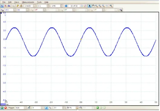
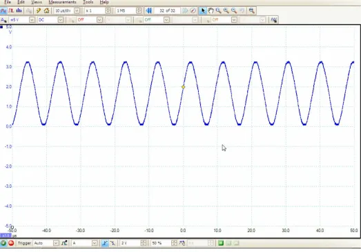
I next entered a small program from the micropython.org DAC tutorial to demonstrate how to generate a sine wave. I named this program DAC_Sine.py and list it here:

(58)

Figure 2-9 400-Hz sine wave.

The output frequency can be altered by changing the integer multiplier located in the write_timed () method. I tried increasing the number and eventually found that the maximum sine wave frequency