Child Fostering Decisions in Burkina Faso
Richard Akresh
a b s t r a c t
Using data I collected in Africa, this paper examines a household’s decision to adjust its size through child fostering, an institution where biological parents temporarily send children to live with other families. Households experiencing negative idiosyncratic income shocks, child gender imbalances, located further from primary schools, or with more ‘‘good’’ quality network members (fewer subsistence farmers and unmarried individuals and more educated members) are significantly more likely to send a child. Results reject an overall symmetric fostering model across senders and receivers, but evidence of symmetry is found when the test is restricted to exogenous income shocks and gender imbalances.
I. Introduction
In sub-Saharan Africa, the social institution of child fostering, in which parents send their biological children to live temporarily with another family, is widespread. Household survey data collected by the author in rural Burkina Faso show that in the year 2000, 15 percent of households either sent or received a child, and 8.3 percent of all children were sent or received in that year. Child fostering is Richard Akresh is an assistant professor in the Department of Economics at the University of Illinois at Urbana-Champaign. The author is grateful to Michael Boozer, Paul Schultz, and Christopher Udry for extensive support and suggestions during the project design, fieldwork, and analysis stages. He also thanks Ilana Redstone Akresh, three anonymous referees, and seminar participants at the BREAD and NEUDC conferences and at Brown, Dartmouth, the World Bank, UC Irvine, University of Montreal, University College London, University of Illinois at Urbana-Champaign, Federal Reserve Bank of Chicago, Tufts, Boston University, Columbia, College of William and Mary, Georgetown, Florida State, and University of Chicago for helpful comments. He acknowledges the collaboration between Yale University and l’Institut Supe´rieur des Sciences de la Population of the University of Ouagadougou that aided the data collection. The fieldwork was funded by the National Science Foundation (Grant No. 0082840), Social Science Research Council, J. William Fulbright Fellowship, National Security Education Program, Institute for the Study of World Politics, and Yale Center for International and Area Studies. Finally, he thanks the members of the field research team, in particular the supervisors, Ouedraogo Touende Bertrand and Hubert Barka Traore. The data used in this article can be obtained beginning May 2010 through April 2013 from Richard Akresh (akresh@illinois.edu).
½Submitted May 2007; accepted: July, 2008
ISSN 022-166X E-ISSN 1548-8004Ó2009 by the Board of Regents of the University of Wisconsin System
not unique to Burkina Faso. Demographic and Health survey data from 16 African countries show that the percentage of households with a foster child ranges from 15 percent in Ghana to 37 percent in Namibia (Vandermeersch 1997).1 Lloyd and Desai (1992) use the same survey data to calculate the percent of children living away from their biological parents and find rates ranging from 5 percent in Burundi to 28 percent in Botswana.
Most international development organizations and many researchers believe fostering has negative consequences for a child’s welfare outcomes (Haddad and Hoddinott 1994; UNICEF 1999; Fafchamps and Wahba 2006). This negative view of fostering is often rationalized by arguing parents reap the benefits of the practice while children shoulder the costs (see Edmonds and Pavcnik 2005 and Suri and Boozer 2007 for a related discussion of parental agency and child labor). This is fur-ther evidenced in a 2002 United Nations Committee on the Rights of the Child report that states, ‘‘The committee recommends that½Burkina Fasourgently take all meas-ures necessary to put a stop to the practice of ‘‘fostering’’ and traditional adoption.’’ In 2002, Burkina Faso’s government, in an effort to reduce fostering, debated a law similar to one already considered by neighboring Mali requiring children younger than 18 to have registration documents to travel outside their natal village.
Understanding why families foster is critical for evaluating the institution’s impact on economic development. Researchers hypothesize that fostering allows biological parents to buffer the costs of raising a child (by being able to send him away tem-porarily) and might be responsible for the persistently high fertility levels seen throughout Africa and the resulting slower economic growth (Bledsoe 1990). How-ever, fostering also provides another mechanism for biological parents to use to smooth consumption in risky environments. Finally, in regions with limited resources for human capital investment, fostering could enable biological parents to move a child to areas where this investment is feasible, which, in turn, might facilitate growth. The existence of this institution affords biological parents a broader choice set of where their children can live; if households make fostering decisions based on economic reasons, then restricting a household’s ability to foster might have unin-tended, negative welfare implications.
In this paper, I present an economic framework and empirical evidence that four principal factors are correlated with a household’s decision to foster a child. First, households that experience exogenous idiosyncratic negative income shocks are more likely to send a child to live with another family. Previous researchers docu-ment that, in risky environdocu-ments, households use various methods to cope with ex-ogenous shocks such as migration and marriage strategies (Rosenzweig and Stark 1989; Paulson 2003), livestock sales (Rosenzweig and Wolpin 1993), informal credit markets (Udry 1994), increased labor supply (Frankenberg, Smith, and Thomas
2003), and transfers from relatives and neighbors (Fafchamps and Lund 2003).2 None of the existing economics research has been able to test whether households respond to transitory idiosyncratic shocks by fostering a child.
Second, in most African households, children perform chores that include cook-ing, cleancook-ing, childcare, getting water, and running errands. Having too many chil-dren of a given gender may not optimize household production, thereby making parents more likely to send a child to offset demographic imbalances. These child labor results are consistent with the seminal economics work on child fostering by Ainsworth (1990; 1996) as well as with research by anthropologists, demographers, and sociologists working in West Africa (Goody 1982; Oppong and Bleek 1982; Isiugo-Abanihe 1985; Bledsoe and Isiugo-Abanihe 1989).
The next two factors relate broadly to a child’s human capital investment. If schooling is not available locally, biological parents might send a child away. Goody (1982), Isiugo-Abanihe (1985), Zimmerman (2003), and Serra (2009) provide evi-dence for this, but Ainsworth (1990) cannot confirm it empirically. Fourth, house-holds with better external opportunities, measured in terms of their social network’s quality, are more likely to send a child. Even if the child does not attend school, being in a better environment may provide access to improved healthcare, better nutrition, more learning opportunities, or greater social mobility and is gener-ally viewed as a positive investment in the child’s future. Previous research considers the role social networks play in finding jobs (Granovetter 1973; Munshi 2003) and migrating (Espinosa and Massey 1997), but the link between social networks and child fostering has never been explored or quantitatively measured.
This paper is part of a broader research program that examines the impact of fos-tering on children’s welfare and is based on Burkina Faso household survey data col-lected by the author. I adopted a methodology that involves locating and interviewing the sending and receiving household of each fostering exchange. For example, if a household interviewed in the initial sample sent a child to another family, then the receiving household was found and interviewed in the survey’s tracking phase. Sim-ilarly, if a household interviewed in the initial sample received a child, then the child’s biological parents (sending household) were located and interviewed. There were 316 paired households to be found during the tracking phase, and the field re-search team located 94.9 percent of them, yielding a total of 300 households.3This is the first time both the sending and receiving households from a given fostering
2. Frankenberg, Smith, and Thomas (2003) examine changes in household size as a mechanism households utilized in response to the 1997 Indonesian financial crisis. Butcher (1993) also finds evidence of household size changing in response to village-level macro characteristics. The focus of those papers on the household response to aggregate, macroeconomic shocks differs from the current analysis’ exclusive focus on the im-pact of idiosyncratic shocks on child fostering. Sociologists and demographers also provide evidence households use fostering to deal with uncertainty and risk (Goody 1982; Bledsoe and Isiugo-Abanihe 1989).
exchange were tracked and interviewed and the tracking’s success makes these data unique.4
Although the tracked households are not used in this paper, they are critical to un-derstanding and measuring the welfare implications of fostering for the foster child, the biological siblings remaining behind, and the host siblings in the receiving house-hold. A related paper (Akresh 2007) using these tracked data measures the impact of child fostering on school enrollment and finds that young foster children are 17.5 and 17.9 percent more likely to be enrolled after fostering compared to their host and bi-ological siblings, respectively.
While the current paper is based on cross-sectional data and is predominantly de-scriptive, identifying which factors are correlated with a household’s decision to send or receive a child is a critical first step in understanding the economics of fostering and using data specifically designed to analyze fostering allows me to explore moti-vations that have not been previously studied in the literature. The two exceptions to the nature of this study being descriptive are the shock variables and the sex ratio variables, both of which I argue could be considered exogenous measures. An unex-pected drop of $100 in household income (approximately one-third of a standard de-viation), when average household income in the sample is $158, increases the probability of sending a child above the current fostering level by 22.6 percent. Like-wise, having more biological girls than boys in the household is correlated with a 39 percent increased probability of sending a girl, while having more biological boys than girls is correlated with a 28 percent increased probability of sending a boy. Re-garding the other measures, I find a significant positive correlation between the dis-tance to the nearest primary school and a household sending a child and a smaller, weaker negative correlation between school distance and a household receiving a child. In addition, measures of the quality of a household’s extended family network are correlated with the likelihood of sending but not receiving a child. In particular, a household with a network that has an educated member, fewer subsistence farmers, fewer unmarried individuals, and more members is more likely to send a child. Fi-nally, I formally test and reject that the four factors (shocks, sex ratios, distance to school, and network quality) correlated with the sending decision have an equal and opposite relationship with the receiving decision. However, if I restrict the test to only the exogenous variables (shocks and sex ratios), I cannot reject that they have an equal and opposite effect on a household’s sending and receiving decision, pro-viding some evidence of symmetry in the fostering decision.
The current paper is most closely related to Zimmerman’s (2003) paper that exam-ines child fostering in South Africa and finds evidence that schooling is important for the receiving decision, but there are three critical points that differentiate these two papers. First, I examine both the household sending and receiving decisions and compare whether the same variables are correlated with each decision. Zimmerman,
due to data limitations, only focuses on the household receiving decision, which also means that comparisons of the factors correlated with sending and receiving a child could not be compared. Second, I use the sex ratios of a household’s biological dren, an arguably more exogenous demographic measure than the number of chil-dren, to examine the relevance of child labor as a predictor of fostering. Third, I consider the relationship between child fostering, extended family network quality, and idiosyncratic shocks. Zimmerman does not have information on a household’s shocks or extended family and so consequently could not explore these factors as motivations for fostering.
The remainder of the paper is organized as follows. Section II describes the em-pirical setting for the data collection. In Section III, I describe in more detail possible motivations for the household fostering decision. Section IV presents the empirical results for the household sending and receiving decision and tests whether the results are symmetric. Section V concludes.
II. Empirical Setting
The data were collected in Bazega province in central Burkina Faso, located approximately 50 miles from the capital.5Households in this region are
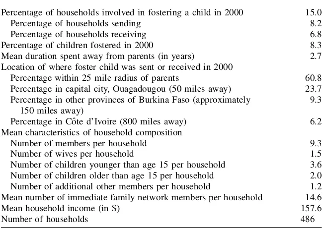
pre-dominantly subsistence farmers growing sorghum and groundnuts and have a mean annual income of $158 (using the average foreign exchange rate in 2000 of $1¼714 FCFA). On average, these households have 9.3 members consisting of a household head, 1.5 wives, 3.6 children younger than age 15, 2.0 children older than age 15, and 1.2 members that might include the household head’s mother, brothers, sisters, grandchildren, and distant relatives. Table 1 contains additional summary statistics for the data.
The project’s fieldwork improves on previous studies in several ways. First, as mentioned above, this is the first data collection to track and interview both the send-ing and receivsend-ing households in a given fostersend-ing exchange. Of the children sent or received in 2000, 61 percent of the paired households were located within a 25-mile radius of the child’s home, 24 percent were located 50 miles away in the capital, 9 percent were scattered across Burkina Faso about 150 miles away, and 6 percent were in Coˆte d’Ivoire approximately 800 miles away.6
Second, I collect detailed information on occupation, marital status, education, and demographic characteristics for every individual in the respondent and his wife’s
5. Additional information about the fieldwork, including the survey instruments, training manuals, and pro-ject reports can be found on the author’s website:Æhttps://netfiles.uiuc.edu/akresh/www/æ.
immediate family network. I limit the network definition to only include immediate family members (parents, brothers, sisters, and adult children) that are not co-resident, instead of all potential households that could send or receive a child.7Restricting the
inclusion of network members has the advantage that the network is then determined prior to any fostering decision (because the network is only direct biological rela-tives) and any potential reverse causality problems related to the correlation of a household’s fostering decision with its choice of network members is reduced. By defining a network as only biological relatives, a potential sending household, in effect, takes its network’s size and quality as given at the time of the fostering de-cision. This is a significant improvement over other studies examining a social net-work’s relationship to household decisions but which rely on respondent reports of
Table 1
Summary Statistics from Burkina Faso Child Fostering Household Survey
Percentage of households involved in fostering a child in 2000 15.0
Percentage of households sending 8.2
Percentage of households receiving 6.8
Percentage of children fostered in 2000 8.3
Mean duration spent away from parents (in years) 2.7
Location of where foster child was sent or received in 2000
Percentage within 25 mile radius of parents 60.8
Percentage in capital city, Ouagadougou (50 miles away) 23.7 Percentage in other provinces of Burkina Faso (approximately
150 miles away)
9.3
Percentage in Coˆte d’Ivoire (800 miles away) 6.2
Mean characteristics of household composition
Number of members per household 9.3
Number of wives per household 1.5
Number of children younger than age 15 per household 3.6 Number of children older than age 15 per household 2.0 Number of additional other members per household 1.2 Mean number of immediate family network members per household 14.6
Mean household income (in $) 157.6
Number of households 486
Note: A child was considered fostered if the child did not live in the same compound with either biological parent, was aged 5-15 inclusive, and had lived away from the biological parents for at least four consecutive months. Data source: Author’s survey.
network members, making the network definition endogenous.8 This information allows me to examine quantitative measures of the network’s quality and the rela-tionship of that quality to the fostering decision, which prior to this data collection was not possible.
Third, I asked retrospective questions about agricultural production and shocks for every crop the household grew to calculate deviations of the current year’s agricul-tural shock from the three-year mean shock (see Rosenzweig and Wolpin 2000 for a discussion of shock deviations).
The fieldwork’s initial phase entailed interviews with 606 household heads and 812 wives in 15 randomly selected villages in Bazega province. The sampling frame’s unit of analysis was the compound, with some compounds containing mul-tiple households.9 Within each compound, an enumerator interviewed each house-hold head and then separately interviewed each of his wives, if applicable. The tracking phase of the survey consisted of finding the paired households that ex-changed a foster child and interviewing each household head and his wives using the same survey instrument as the initial phase. A child was considered fostered if the child did not live in the same compound with either biological parent, was aged 5-15 inclusive, and had lived away from the biological parents for at least four con-secutive months.10
III. Motivations for Child Fostering
To explore a household’s motivation for fostering, I consider the im-portance of risk-coping, child labor, schooling, and network quality. In this frame-work, I examine each motivation in isolation, although in reality and in the
8. Although a potential sending household does not choose which households are in its network at the time of the fostering decision, these immediate family networks are not exogenously determined. In the distant past, residency decisions with siblings and adult children and the addition of a spouse’s immediate family network at the time of marriage were choice variables and those past decisions might be correlated with current fostering decisions, although these are likely to be second-order concerns and are not issues I can address with these data.
9. To increase the sample of fostering households, I used a two-part sampling frame that included a random and a choice-based sample both drawn from a village level census with information about every house-hold’s fostering status (see Akresh 2004 for details). The choice-based sample consisted of compounds that fostered a child between 1998 and 2000. All results in the paper use the entire sample, but results are quan-titatively similar when restricted to the random sample. Using the population fostering weights from the village level census to adjust the choice-based sample does not significantly alter the results. A total of 383 compounds containing 606 households were selected with 60.7 percent of the compounds in the ran-dom sample.
empirical analysis, the relationship between fostering and these motivations is con-sidered jointly.
First, I consider the risk-coping explanation, assuming there is no fostering for la-bor productivity or educational reasons. I assume household production does not de-pend on child labor. In this setting, there are no insurance or financial markets, but fostering acts as an insurance substitute (see Besley 1995 and Morduch 1995 for a discussion of nonmarket institutions serving as insurance substitutes). Households in a network will try to equalize the marginal utility of consumption across states of nature by fostering children. In other words, if a household experiences an adverse shock and subsequent low consumption, it will send a child to a household in the network experiencing high consumption, thereby reducing its own expenses for the child’s food, clothing, and healthcare. Testing this hypothesis requires measures of transitory, idiosyncratic shocks for the household.
Second, I consider the labor productivity explanation, assuming there is no foster-ing for risk-copfoster-ing or schoolfoster-ing reasons. I assume perfect insurance markets, so households have complete insurance. In this scenario, children provide labor for household production in the form of chores or farm work. For a given age range and gender, most children will perform nearly identical tasks. However, in contrast with other developing countries (Fafchamps 1993; Edmonds and Sharma 2005), adult and child labor markets are nonexistent in rural Burkina Faso. For a given pro-duction function, a family with multiple children of the same gender and age range will have a lower marginal productivity of their labor than a family with few chil-dren. Even with perfect insurance markets, a household fosters children to equalize the marginal product of child labor across the network’s households. Testing this child labor hypothesis requires detailed demographic measures of the age and gender of a household’s children.
Third, I consider educational investment as a possible motivation and assume there is no fostering for risk-coping or child labor reasons. I assume there are perfect in-surance markets and children are not involved in household production. In many de-veloping countries, as in Burkina Faso, children are a form of social security when parents are old. Investing in a child’s education is expected to increase the child’s earning potential. Then, when the child is an adult, transfers are made to the biolog-ical parents in return for the schooling investment (Cox 1987). Testing this schooling hypothesis requires information on school availability and quality.
These factors (risk-coping, child labor, schooling, and network quality) could ex-plain child sending and receiving decisions for a household. A household that expe-riences a bad shock, has child demographic imbalances, is located far from a school, or has many ‘‘good’’ quality network members might be more likely to send a child, while a household that has a good shock (or a less negative one), has fewer imbal-ances in child demographics, is located near a school, or has many ‘‘low’’ quality network members might be more likely to receive a child.
IV. Empirical Results
A. Preliminary Observations
To explore the relationship between shocks, child demographics, school availability, and network quality and the household sending and receiving decisions, in Table 2, I present conditional means for each of the variables broken down by whether the household sent a child, received a child, or did neither. Note that all 486 households in the analysis are located in the 15 randomly selected rural villages, so any differ-ences observed in the conditional means (for example, the distance to a primary school or income shocks for a sending versus a receiving household) cannot be due to factors such as rural-urban differences. Of the 486 households, 8.2 percent sent a child and 6.8 percent received a child.
The shock measures build on sociological hypotheses that economic crises impact a household’s decision to send a child (Jonckers 1997). I calculate two distinct shock measures, with the first based on agricultural events and the second based on income. Because the survey respondents are rural, subsistence farmers, their economic envi-ronment and relevant crises are well captured by measures of agricultural shocks. To measure these shocks, I use the response to the question, ‘‘For each crop grown in a given year, how much of that crop was lost due to an unexpected agricultural event?’’ Answers are coded from zero (no loss) to three (large loss). To help individuals respond, enumerators provide examples of unexpected agricultural events such as animals running through the respondent’s fields; pest, rodent, or fungus infestations; or unexpected localized weather damage such as hail. I calculate the household ag-ricultural shock as the household’s current year’s shock (mean of all that year’s crop-specific shocks) minus the three-year household average, with a larger value indicat-ing a more negative shock. The measure explicitly takes into account a household’s shock history and varies across households in a village. The mean household agricul-tural shock is 0.446, but sending households experience a worse average shock of 0.603, while receiving households experience a smaller shock of 0.506.11
I calculate similarly the household income shock as the three-year average house-hold income minus current househouse-hold income, with a larger value indicating a more negative shock. Sending households, on average, experience a negative income shock of 0.181 (current income below average household income), while receiving
Table 2
Conditional Means and Standard Deviations for Household Level Characteristics
Variables
Household income shock 0.051 0.181 0.044 20.008
(0.583) (0.679) (0.582) (0.443)
Number of householdsa 486 40 415 33
households experience a small positive income shock of -0.008 (current income above average household income). Using income shocks is advantageous because they allow for the possibility of positive shocks, are easy to interpret, and I can ex-amine the relationship between a percentage change in household income and child fostering. However, income changes can also incorporate household labor supply adjustments in response to an exogenous shock and therefore could be considered endogenous, which is why I present both income shocks as well as agricultural shocks in the regression analysis.
To examine if demographic imbalances in the gender composition of a hold’s biological children are correlated with the fostering decision, for each house-hold I create a variable indicating if the househouse-hold has equal numbers of boys and girls, more girls than boys, or more boys than girls. I use this gender imbalance vari-able, an arguably more exogenous measure of household demographics, to examine the child labor issue. Sociologists argue that having too many or too few children of a particular gender and age are situations where a household may respectively send or receive a child to address the excess or deficit (Jonckers 1997). Sending households are more likely to exhibit gender imbalances, with more girls than boys or more boys than girls, while receiving households are more likely to have the same number of boys and girls.
The distance to the nearest primary school proxies for a child’s educational oppor-tunities and indicates that sending households live further from schools (2.09 kilo-meters) than receiving households (1.58 kilokilo-meters). Of the 15 randomly selected rural villages in which these 486 households reside, eight of the villages have a pri-mary school while seven do not.
To explore whether network characteristics are correlated with a household’s fos-tering decision, I examine network size plus four distinct network quality measures. Sending households have 16.13 immediate family members while receiving house-holds have 17.94. This contrasts with nonfostering househouse-holds who have smaller net-works with only 14.20 members.
Conditional on a household’s network size, the characteristics of the network members might be critically related to the fostering decision, with households with more ‘‘good’’ quality members more likely to send and less likely to receive a child. I examine occupation, education, marital status, and fostering history of the previous generation. First, sending households have 9.65 farmers and receiving households have 12.21 in their extended family network. While I do not have income data for each network member, using the respondent’s occupation and income, I find a strong correlation between farming and lower income. If a smaller fraction of the network is low income members, then conversely more of the network has a good occupation with higher income, which is helpful for a household that wants to send a child. For receiving households, this implies there are more network members who might want to send a child.
stable marital situations, which is conducive to sending a child, while the converse for receiving is also true.
Fourth, I explore the relationship between current fostering of children and the fos-tering history of the network members when they were children by creating a vari-able indicating if any immediate family member had been fostered as a child. The fraction of households with a network member who had been fostered as a child is lower in sending than receiving households. This may be a signal the network is of low quality. In other words, having an extended family network in which mem-bers had been fostered as children might indicate a network that had previously ex-perienced negative income shocks.
B. Household Sending Decision
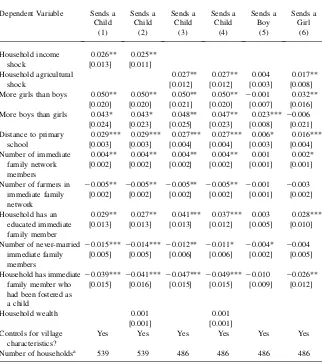
In Table 3, I present results examining the correlates of the household sending deci-sion using a logit model where the dependent variable equals one if a household sent a child aged 5-15 (inclusive) and zero otherwise, and the explanatory variables mea-sure the household’s idiosyncratic income or agricultural shocks, child gender imbal-ances, distance to the nearest primary school, and network quality.12 Empirical
results are consistent with previously discussed motivations. A household is more likely to send a child if it experiences a worse income or agricultural shock, has de-mographic imbalances in the gender composition of its children, lives further from a primary school, or has a better quality network of potential receivers.13
A one-unit increase in a household’s income shock (equal to a 100,000 FCFA or $140 USD decline in income) is correlated with a 2.6 percent increase in the house-hold probability of sending a child (Column 1), a relationship that is statistically sig-nificant at the 5 percent level. This is robust to the inclusion of household wealth (Column 2). With 8.2 percent of households sending a child, a one standard deviation increase in a household’s income shock (Column 1) is correlated with an 18.5 per-cent increase in the likelihood of sending. Alternatively, a ten perper-cent drop from the mean in household income (approximately 0.2 standard deviations) yields a 3.6 percent increase in the likelihood of sending.14
Similar results are obtained in Columns 3 and 4 using a household’s agricultural shock instead of income shock. A one standard deviation increase in a household’s agricultural shock raises the probability a household sends a child by 1.8 percent and is statistically significant at the 5 percent level. Relative to the base sending level, a one standard de-viation agricultural shock increase leads to a 22.5 percent increase in sending.
12. All regressions also include village characteristics (presence of a weekly market, health clinic, animal traction availability, village’s main water source, number of months with a reliable water source, and village religion) to control for factors unique to each village.
13. To exploit additional information from households sending multiple children, I also estimate the send-ing decision with an ordered logit in which the dependent variable is the number of children a household sent. Results are similar because 91.8 percent of households sent no child, 7.0 percent sent one child, and only 1.2 percent sent two children.
The biological child gender imbalance variables indicate that a household with more girls than boys or more boys than girls has a higher probability of sending a child compared to households with the same number of boys and girls. Having more
Table 3
Marginal Effects from Household Level Logit Regressions Estimating the Probability of Sending a Child More girls than boys 0.050** 0.050** 0.050** 0.050** 20.001 0.032**
[0.020] [0.020] [0.021] [0.020] [0.007] [0.016] More boys than girls 0.043* 0.043* 0.048** 0.047** 0.023*** 20.006
[0.024] [0.023] [0.025] [0.023] [0.008] [0.021] Distance to primary
school
0.029*** 0.029*** 0.027*** 0.027*** 0.006* 0.016*** [0.003] [0.003] [0.004] [0.004] [0.003] [0.004] Number of immediate
family network members
0.004** 0.004** 0.004** 0.004** 0.001 0.002* [0.002] [0.002] [0.002] [0.002] [0.001] [0.001]
Number of farmers in immediate family network
20.005** 20.005** 20.005** 20.005** 20.001 20.003
[0.002] [0.002] [0.002] [0.002] [0.001] [0.002]
Household has an educated immediate family member
0.029** 0.027** 0.041*** 0.037*** 0.003 0.028*** [0.013] [0.013] [0.013] [0.012] [0.005] [0.010]
Number of never-married immediate family members
20.015*** 20.014***20.012** 20.011* 20.004* 20.004
[0.005] [0.005] [0.006] [0.006] [0.002] [0.005]
Household has immediate
Yes Yes Yes Yes Yes Yes
Number of householdsa 539 539 486 486 486 486
Note: Robust standard errors in brackets, clustered at village level. * significant at 10 percent; ** significant at 5 percent; *** significant at 1 percent. See Table 2 for variable definitions. Village characteristics include presence of a weekly market, health clinic, animal traction availability, village’s main water source, number of months with a reliable water source, and village religion. Data source: Author’s survey.
biological girls than boys is correlated with a 5.0 percent increase in the sending probability and the coefficient is significant at the 5 percent level (using either in-come or agricultural shocks and with or without household wealth). Households with more biological boys than girls are 4.3 to 4.8 percent more likely to send a child and the coefficients are significant at the 10 and 5 percent levels respectively depending on whether the regression includes income shocks or agricultural shocks. Results are consistent with the claim that a household uses fostering to cope with a redundancy or an excess of children in a particular demographic category.
The coefficient for the distance to the nearest primary school is positive and sig-nificant at the 1 percent level. Being one kilometer further from a primary school is correlated with a 2.7 to 2.9 percent increased probability of sending a child. Relative to baseline sending rates, a one standard deviation increase in the distance to the nearest school (using the Column 3 coefficients) is correlated with a 64.9 percent in-crease in a household’s sending probability.15
Table 3 also provides evidence that a household with a larger and better quality network is more likely to send a child. Households with more immediate family net-work members are more likely to send a child and the coefficient is significant at the 5 percent level across the Column 1 to 4 specifications. An additional network mem-ber is correlated with a 0.4 percent increase in the sending probability. Having more potential receiving households is important for the sending decision, but the quality of those households is also critical. An additional farmer (a lower income occupa-tion) in a household’s network is correlated with a 0.5 percent lower sending prob-ability and the coefficients are significant at the 5 percent level, but having an educated network member (someone who ever attended school) is correlated with a 2.7 to 4.1 percent increased probability of sending a child. Having an additional never-married network member, a person who cannot provide a stable marital envi-ronment in which to raise a foster child, is correlated with a 1.1 to 1.5 percent lower sending probability. Likewise, having an immediate family member who had been fostered as a child is correlated with a 3.9 to 4.9 percent lower sending probability. I interpret this as an indicator the household’s overall network is of low quality. Al-though I do not have information about the direct cause of the immediate family member’s childhood fostering, it could have been related to an income shock that the immediate family suffered or it could be related to other negative unmeasured factors about the extended family that led them to foster in the past.16Controlling for network size, a household with more ‘‘good’’ quality network members (fewer subsistence farmers, more educated individuals, fewer unmarried individuals, and no members fostered as children) is more likely to send a child.17
Finally, there does not appear to be a strong relationship between household wealth (calculated as the value of the household’s livestock and assets) and a
15. I estimate sending regressions (results not shown) using alternative school measures (presence of a pri-mary school in the village, number of grades in the school, and the year the school was opened) and results are similar.
16. If the immediate family member had been fostered as a child for a longer duration, indicating a more permanent household shock, the sending probability is even lower.
household’s decision to send a child.18Results (in Columns 2 and 4) for shocks, de-mographics, distance to a school, and network quality are robust to the inclusion of wealth measures.19The wealth measures are not statistically significant and in both regressions are close to zero, indicating household permanent characteristics are not important for the sending decision.20
To explore the relationship between a child’s gender and fostering motivations, I estimate household sending regressions broken down by the sent child’s gender. In Column 5, the dependent variable equals one if a household sent a boy aged 5-15 and zero otherwise; in Column 6, the dependent variable equals one if a household sent a girl aged 5-15 and zero otherwise. Results are distinct for boys and girls. First, household agricultural shocks are significant determinants only of the decision to send a girl but not a boy. With 5.6 percent of households sending a girl, a one stan-dard deviation increase in a household’s agricultural shock is correlated with a 20.8 percent increase in the probability of sending a girl.21Second, excess children of a given gender are correlated with an increased probability of sending a child of the same gender. Households with more girls than boys are 3.2 percent more likely to send a girl, while households with more boys than girls are 2.3 percent more likely to send a boy. Third, the correlation between the distance to a primary school and the probability of sending a girl is 2.7 times larger than the same correlation with the probability of sending a boy. Fourth, there is no evidence that network quality is lated to the decision to send a boy, but there is limited evidence that it might be re-lated to the decision to send a girl, with a positive correlation between sending a girl and having an educated immediate family member.
C. Robustness Specifications
To confirm the robustness of the previous results, in results not reported, I estimate four alternative specifications of the sending regressions. First, I estimate the sending regressions using the current year’s direct agricultural events measure (from which I calculate the household agricultural shock) and results are consistent. A household that experiences more unexpected bad agricultural events in the current year is more likely to send out a child, confirming that the previous shock results are not depen-dent on taking into account a household’s shock history.
18. Assets include items typically owned by rural households, such as a bicycle, wheelbarrow, or cart. To account for asset quality heterogeneity, each item’s value as reported by the respondent is used to calculate total asset value.
19. To test if the shock impact varies by household wealth, I include an interaction of wealth and shocks, but results are inconclusive. Similarly, interacting network quality measures and shocks yields insignificant results.
20. In results not reported, I estimate a two-step instrumental variables logit using characteristics of the respondent’s parents as instruments for household wealth, but wealth is still insignificant. In the first step, household wealth is instrumented for and in the second step I estimate a sending logit and include the first stage residuals (Smith and Blundell 1986; Rivers and Vuong 1988). The instruments include the number of wives of the respondent’s father, the rank of the respondent’s mother among the father’s wives, the number of children of the respondent’s father, the number of children of the respondent’s mother, and village-level positions held by either the father or mother.
Second, I estimate a sending regression including village fixed effects to address the issue that variables such as shocks or network quality might be correlated at the village level. Results are consistent with previous regressions that showed a positive relationship between sending a child and shocks, gender imbalances and network quality measures. As the distance to the nearest school variable does not vary within a village, it cannot be included in the village fixed effects regression, and so I cannot examine the relationship between schooling and fostering.
Third, I estimate sending regressions using alternative sample specifications. There were 67 household heads (of 606 households) absent during part of the field-work, so I do not have their individual information on shocks or income, but I have their household demographics, network quality, and distance to school. I include these 67 households in the regressions and assume they experience no income or ag-ricultural shock, and results are consistent both for the shock variables as well as the gender imbalance, school distance, and network quality measures.
Fourth, to examine whether the four motivations have a differential relationship with the decision to send a child to an immediate family member versus a non-relative, I estimate a multinomial logit in which the dependent variable represents no child sent, child sent to an immediate family member, or child sent to a non-relative. There are differences in factors predicting sending to immediate family versus nonrelatives. I find that a household experiencing a negative agricultural shock is significantly more likely to send a child to a nonrelative, while there is no relationship between shocks and sending to an immediate family member. On the other hand, gender imbalances and distance to school are only correlated with the decision to send a child to an immediate family member and not a non-relative.
D. Household Receiving Decision
Table 4
Marginal Effects from Household Level Logit Regressions Estimating the Probability of Receiving a Child
Household income shock20.003 20.004 [0.005] [0.005]
[0.026] [0.025] [0.026] [0.025] [0.009] [0.013] More boys than girls 20.019 20.020 20.028 20.029 0.006 20.021**
[0.022] [0.023] [0.024] [0.024] [0.012] [0.010] Distance to primary
school
20.006*20.006*20.003 20.003 20.004 20.000 [0.003] [0.003] [0.003] [0.003] [0.003] [0.002] Number of immediate
family network members
0.001 0.001 0.002 0.002 0.001 0.001 [0.002] [0.002] [0.002] [0.002] [0.001] [0.001]
Number of farmers in immediate family network
0.001 0.001 0.001 0.000 0.000 0.000 [0.002] [0.002] [0.002] [0.002] [0.001] [0.001]
Household has an educated immediate family member
0.012 0.010 0.015 0.012 0.015*20.002 [0.012] [0.012] [0.011] [0.011] [0.008] [0.007]
Number of never-married immediate family members
20.002 20.001 20.004 20.003 20.003 20.002 [0.004] [0.004] [0.005] [0.005] [0.003] [0.002]
Household has immediate
Yes Yes Yes Yes Yes Yes
Number of householdsa 539 539 486 486 486 486
Note: Robust standard errors in brackets, clustered at village level. * significant at 10 percent; ** significant at 5 percent; *** significant at 1 percent. See Table 2 for variable definitions. Village characteristics include presence of a weekly market, health clinic, animal traction availability, village’s main water source, number of months with a reliable water source, and village religion. Data source: Author’s survey.
E. Jointly Testing Sending and Receiving Decisions
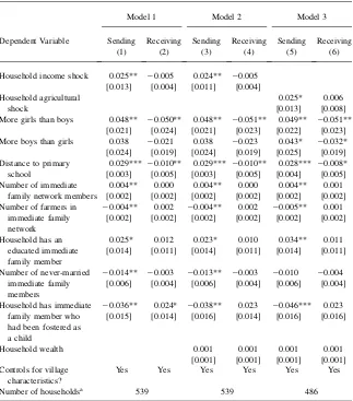
The sending and receiving regressions in Tables 3 and 4 provide preliminary evi-dence that the same variables are not correlated with both decisions. However, part of why the regressions are not mirror images is explained by the sample’s nonfoster-ing households. In the sendnonfoster-ing regression, senders are compared to the group of non-fostering and receiving households, while in the receiving regression, receivers are compared to the group of nonfostering and sending households. To test the hypoth-esis that the factors correlated with the sending decision have an equal and opposite relationship with the receiving decision, I use a multinomial logit regression to esti-mate the probability a household sends a child, receives a child, or does neither. The dependent variable takes the value no fostering for 85.6 percent of households, send-ing for 8.0 percent, and receivsend-ing for 6.4 percent.22
In Table 5, I present the results for three different multinomial logit models that differ in whether they include income shocks, agricultural shocks, or household wealth. Across the three models, the sending outcome coefficients (Columns 1, 3, and 5) for shocks, demographics, distance to school, and network quality are similar in magnitude and significance to the Table 3 sending results. However, the receiving outcome coefficients (Columns 2, 4, and 6) for the gender imbalance and distance to the nearest primary school variables are now statistically significant at the 5 percent level. Households with more girls than boys are 5.0 to 5.1 percent less likely to re-ceive a child compared to a nonfostering household, while being one kilometer fur-ther from a primary school is correlated with a 0.8 to 1.0 percent reduced probability of receiving a child. There is still no statistically significant relationship between re-ceiving a child and either shocks or network quality measures. Likewise, household wealth is not correlated with either the sending or receiving decisions.
To formally test the symmetry hypothesis of whether the household sending and receiving decisions are correlated with the same variables in an equal and opposite way, I calculate a Wald test of the joint restriction that the coefficients for the shocks, gender imbalances, distance to a primary school, and network quality variables for the sending outcome are equal and opposite to the coefficients for the receiving outcome. Across all models, I can reject the symmetry hypothesis for the four motivations jointly. However, for the distance to the nearest school variable, while I reject that the sending coefficient is the same magnitude as the receiving coefficient, they are clearly opposite in sign with households further from a school more likely to send and less likely to receive a child. Finally, if I restrict the symmetry test to only include the arguably exogenous variables (household shocks and child gender demographic imbalances), then I cannot reject the equal and opposite symmetry hypothesis, provid-ing evidence that a symmetric model might explain some child fosterprovid-ing motivations.
V. Conclusion
In this paper, using household survey data I collected in West Africa, I analyze a household’s decision to change its size and composition by sending or
receiving children. The practice of biological parents temporarily sending a child to live with another family constitutes a long-standing and widespread social institution in Africa. I find that households that experience negative idiosyncratic income
Table 5
Marginal Effects from Household Multinomial Logit Regression Estimating Probability of Sending, Receiving, or No Fostering
Model 1 Model 2 Model 3
Dependent Variable Sending Receiving Sending Receiving Sending Receiving
(1) (2) (3) (4) (5) (6)
Household income shock 0.025** 20.005 0.024** 20.005
[0.013] [0.004] [0.011] [0.004] Household agricultural
shock
0.025* 0.006 [0.013] [0.008] More girls than boys 0.048** 20.050** 0.048** 20.051** 0.049** 20.051**
[0.021] [0.024] [0.021] [0.023] [0.022] [0.023] More boys than girls 0.038 20.021 0.038 20.023 0.043* 20.032*
[0.024] [0.019] [0.024] [0.019] [0.025] [0.019] Distance to primary
school
0.029*** 20.010** 0.029*** 20.010** 0.028*** 20.008*
[0.003] [0.005] [0.003] [0.005] [0.004] [0.005] Number of immediate
family network members
0.004** 0.000 0.004** 0.000 0.004** 0.001 [0.002] [0.002] [0.002] [0.002] [0.002] [0.002] Number of farmers in
immediate family network
20.004** 0.002 20.004** 0.002 20.005** 0.001
[0.002] [0.002] [0.002] [0.002] [0.002] [0.002]
Household has an educated immediate family member
0.025* 0.012 0.023* 0.010 0.034** 0.011 [0.014] [0.011] [0.014] [0.011] [0.014] [0.011]
Number of never-married immediate family members
20.014** 20.003 20.013** 20.003 20.010 20.004
[0.006] [0.004] [0.006] [0.004] [0.006] [0.004]
Household has immediate
Household wealth 0.001 0.001 0.001 0.001
[0.001] [0.001] [0.001] [0.001] Controls for village
characteristics?
Yes Yes Yes Yes Yes Yes
Number of householdsa 539 539 486
Note: Robust standard errors in brackets, clustered at village level. * significant at 10 percent; ** significant at 5 percent; *** significant at 1 percent See Table 2 for variable definitions. Village characteristics include presence of a weekly market, health clinic, animal traction availability, village’s main water source, number of months with a reliable water source, and village religion. Data source: Author’s survey.
shocks or child demographic gender imbalances are significantly more likely to send out a child. A ten percent drop in household income is associated with a 3.6 percent increased likelihood of sending a child, while having more biological girls than boys is correlated with a 39 percent increased probability of sending a girl. There is also a strong correlation between a household’s distance to the nearest primary school and the fostering decision, with households further from a school more likely to send and less likely to receive a child. Finally, I find that a household with more ‘‘good’’ qual-ity extended family network members (fewer subsistence farmers, more educated members, and fewer never-married individuals) is more likely to send a child.
The research methodology and survey design make these unique data well-suited for examining factors correlated with a household’s fostering decision that previous researchers were unable to consider. In particular, this is the first paper to provide empirical evidence that households experiencing adverse shocks use child fostering as a risk-coping mechanism. It is also the first paper to use biological child gender imbalances as an exogenous demographic measure to examine child labor motiva-tions for fostering. Finally, it is the first paper to quantitatively explore the relation-ship between social networks and child fostering. Future research can extend this analysis to explore the relationship between social networks and foster children’s ed-ucation and health outcomes.
Understanding why households engage in this social institution has significant pol-icy implications for international development organizations who are currently trying to prevent children from growing up away from their biological parents. Related re-search using the tracked household data from this project suggests foster children are not negatively affected in terms of school enrollment in either the short-run or long-run by living away from their biological parents (Akresh 2007). If child fostering insulates households from adverse shocks, provides them access to the benefits of extended family networks and additional human capital investment, and moves chil-dren to households where they are more productive, then restricting the movement of children as a policy prescription should be reevaluated. The prevalence of child fos-tering as a means for a household to adjust its structure suggests it is also critical for governments and development organizations, in designing and evaluating policies, to allow for the possibility that a household changes its size in response to government programs (Edmonds, Mammen, and Miller 2005). Further, whenever household size and composition are choices, researchers and practitioners need to consider the po-tential biases arising from endogenous household structure.
References
Ainsworth, Martha. 1990. ‘‘The Demand for Children in Coˆte d’Ivoire: Economic Aspects of Fertility and Child Fostering.’’ Dissertation. New Haven, Conn.: Yale University. __________. 1996. ‘‘Economic Aspects of Child Fostering in Coˆte d’Ivoire.’’ InResearch in
Population Economics, ed. T. Paul Schultz, 25–62. Greenwich: JAI Press Inc. Akresh, Richard. 2004. ‘‘Survey and Tracking Methodology, Fieldwork Definitions, and
Project Overview.’’ Ph.D. Dissertation, Chapter 2. New Haven, Conn.: Yale University. __________. 2007. ‘‘School Enrollment Impacts of Nontraditional Household Structure.’’
University of Illinois at Urbana-Champaign. Unpublished.
Beegle, Kathleen, Joachim De Weerdt, and Stefan Dercon. 2006. ‘‘Orphanhood and the Long-Run Impact on Children.’’American Journal of Agricultural Economics88(5):1266–72. Besley, Timothy. 1995. ‘‘Nonmarket Institutions for Credit and Risk Sharing in Low-Income
Countries.’’Journal of Economic Perspectives9(3):115–27.
Bledsoe, Caroline. 1990. ‘‘The Politics of Children: Fosterage and the Social Management of Fertility Among the Mende of Sierra Leone.’’ InBirths and Power: Social Change and the Politics of Reproduction, ed. W. Penn Handwerker, 81-100. Boulder: Westview Press. Bledsoe, Caroline, and Uche Isiugo-Abanihe. 1989. ‘‘Strategies of Child Fosterage among
Mende Grannies in Sierra Leone.’’ InReproduction and Social Organization in Sub-Saharan Africa, ed. Ron Lesthaeghe, 442-74. Berkeley: University of California Press. Butcher, Kristin. 1993. ‘‘Household Size, Changes in Household Size, and Household
Responses to Economic Conditions: Evidence from the Coˆte d’Ivoire.’’ Ph.D. Dissertation, Chapter 3. Princeton, N. J.: Princeton University.
Cox, Donald. 1987. ‘‘Motives for Private Income Transfers.’’Journal of Political Economy 95(3):508–46.
Edmonds, Eric, Kristin Mammen, and Douglas Miller. 2005. ‘‘Rearranging the Family? Income Support and Elderly Living Arrangements in a Low Income Country.’’Journal of Human Resources40(1):186–207.
Edmonds, Eric, and Nina Pavcnik. 2005. ‘‘Child Labor in the Global Economy.’’Journal of Economic Perspectives18(1):199–220.
Edmonds, Eric, and Salil Sharma. 2006. ‘‘Institutional Influences on Human Capital Accumulation: Micro Evidence from Children Vulnerable to Bondage.’’ Dartmouth, N. H.: Dartmouth College. Unpublished.
Espinosa, Kristin, and Douglas S. Massey. 1997. ‘‘Undocumented Migration and the Quantity and Quality of Social Capital.’’Soziale Welt12:141–62.
Fafchamps, Marcel. 1993. ‘‘Sequential Labor Decisions Under Uncertainty: An Estimable Household Model of West African Farmers.’’Econometrica, 61(5):1173–97.
Fafchamps, Marcel, and Susan Lund. 2003. ‘‘Risk-sharing Networks in Rural Philippines.’’ Journal of Development Economics71(2):261–287.
Fafchamps, Marcel, and Jackline Wahba. 2006. ‘‘Child Labor, Urban Proximity, and Household Composition.’’Journal of Development Economics79(2):374–97.
Frankenberg, Elizabeth, James P. Smith, and Duncan Thomas. 2003. ‘‘Economic Shocks, Wealth, and Welfare.’’Journal of Human Resources38(2):280–321.
Goody, Esther N. 1982.Parenthood and Social Reproduction: Fostering and Occupational Roles in West Africa.Cambridge: Cambridge University Press.
Granovetter, Mark S. 1973. ‘‘The Strength of Weak Ties.’’American Journal of Sociology 78(6):1360–80.
Haddad, Lawrence, and John Hoddinott. 1994. ‘‘Household Resource Allocation in the Coˆte d’Ivoire: Inferences from Expenditure Data.’’ InPoverty, Inequality, and Rural
Isiugo-Abanihe, Uche. 1985. ‘‘Child Fosterage in West Africa.’’Population and Development Review11(1):53–73.
Jonckers, Danielle. 1997. ‘‘Les Enfants Confie´s.’’ InMe´nages et Familles en Afrique, ed. Marc Pilon, The´re`se Locoh, Emilien Vignikin, Patrice Vimard, 193-208. Paris: Centre Francxais sur la Population de le De´veloppement.
Lloyd, Cynthia B., and Sonalde Desai. 1992. ‘‘Children’s Living Arrangements in Developing Countries.’’Population Research and Policy Review11(3):193–216.
Moehling, Carolyn M. 2002. ‘‘Broken Homes: TheÔMissingÕChildren of the 1910 Census.’’ Journal of Interdisciplinary History33(2):205–33.
Morduch, Jonathan. 1995. ‘‘Income Smoothing and Consumption Smoothing.’’Journal of Economic Perspectives9(3):103–14.
Munshi, Kaivan. 2003. ‘‘Networks in the Modern Economy: Mexican Migrants in the U.S. Labor Market.’’Quarterly Journal of Economics118(2):549–99.
Oppong, Christine, and Wolf Bleek. 1982. ‘‘Economic Models and Having Children: Some Evidence from Kwahu, Ghana.’’Africa52(4):15–33.
Paulson, Anna. 2003. ‘‘Insurance Motives for Migration: Evidence from Thailand.’’ Chicago: Federal Reserve Bank of Chicago. Unpublished.
Rivers, Douglas, and Quang H. Vuong. 1988. ‘‘Limited Information Estimators and Exogeneity Tests for Simultaneous Probit Models.’’Journal of Econometrics39(3): 347–66.
Rosenzweig, Mark R. and Oded Stark. 1989. ‘‘Consumption Smoothing, Migration, and Marriage: Evidence from Rural India.’’Journal of Political Economy97(4):905–26. Rosenzweig, Mark R., and Kenneth Wolpin. 1993. ‘‘Credit Market Constraints, Consumption
Smoothing, and the Accumulation of Durable Production Assets in Low-Income Countries: Investments in Bullocks in India.’’Journal of Political Economy101(2):223–44. __________. 2000. ‘‘NaturalÔNatural ExperimentsÕin Economics.’’Journal of Economic
Literature38(4):827–74.
Serra, Renata. 2009. ‘‘Child Fostering in Africa: When Labor and Schooling Motives May Coexist.’’Journal of Development Economics88(1):157–70.
Smith, Richard, and Richard Blundell. 1986. ‘‘An Exogeneity Test for a Simultaneous Equation Tobit Model with an Application to Labor Supply.’’Econometrica54(3):679–85. Suri, Tavneet, and Michael Boozer. 2007. ‘‘Child Labor and Schooling Decisions in Ghana.’’
Cambridge: MIT Sloan. Unpublished.
Thomas, Duncan, Elizabeth Frankenberg, and James P. Smith. 2001. ‘‘Lost But Not Forgotten: Attrition and Follow-Up in the Indonesian Family Life Survey.’’Journal of Human Resources36(3):556–92.
Udry, Christopher. 1994. ‘‘Risk and Insurance in a Rural Credit Market: An Empirical Investigation in Northern Nigeria.’’Review of Economic Studies61(3):495–526. UNICEF. 1999. ‘‘Child Domestic Work.’’ Innoncenti Digest, No. 5. International Child
Development Center. Florence, Italy.
Vandermeersch, Ce´line. 1997. ‘‘Les Enfants Confie´s Au Se´ne´gal.’’ Colloque Jeune Chercheurs, INED. May 12–14.
__________. 2002. ‘‘Child Fostering Under Six in Senegal in 1992-1993.’’ Population-English57(4-5):659–86.