Full Terms & Conditions of access and use can be found at
http://www.tandfonline.com/action/journalInformation?journalCode=ubes20
Download by: [Universitas Maritim Raja Ali Haji] Date: 12 January 2016, At: 23:41
Journal of Business & Economic Statistics
ISSN: 0735-0015 (Print) 1537-2707 (Online) Journal homepage: http://www.tandfonline.com/loi/ubes20
Estimating Housing Demand With an Application
to Explaining Racial Segregation in Cities
Patrick Bajari & Matthew E Kahn
To cite this article: Patrick Bajari & Matthew E Kahn (2005) Estimating Housing Demand With
an Application to Explaining Racial Segregation in Cities, Journal of Business & Economic Statistics, 23:1, 20-33, DOI: 10.1198/073500104000000334
To link to this article: http://dx.doi.org/10.1198/073500104000000334
View supplementary material
Published online: 01 Jan 2012.
Submit your article to this journal
Article views: 400
View related articles
Estimating Housing Demand With an Application
to Explaining Racial Segregation in Cities
Patrick BAJARI
Department of Economics, Duke University and National Bureau of Economic Research, Durham, NC 27708 (bajari@econ.duke.edu)
Matthew E. K
AHNTufts University, Medford, MA 02155 (matt.kahn@tufts.edu)
We present a three-stage, nonparametric estimation procedure to recover willingness to pay for housing attributes. In the first stage we estimate a nonparametric hedonic home price function. In the second stage we recover each consumer’s taste parameters for product characteristics using first-order conditions for utility maximization. Finally, in the third stage we estimate the distribution of household tastes as a func-tion of household demographics. As an applicafunc-tion of our methods, we compare alternative explanafunc-tions for why blacks choose to live in center cities while whites suburbanize.
KEY WORDS: Demand estimation; Hedonics; Heterogeneity; Nonparametrics; Product differentiation; Racial segregation.
1. INTRODUCTION
Housing accounts for a major fraction of consumer spend-ing and wealth. Shelter is the largest of the seven categories that comprise the consumer price index (CPI) market basket, accounting for 32% of the total index. Between 1935 and 1991, shelter’s budget share increased by 61%, while food’s budget share fell by 59% (Costa 1998). Housing equity represents the largest source of household wealth. Based on the 1998 Survey of Consumer Finances, the value of stocks owned by house-holds was $7.8 trillion, whereas the value of primary residences was $9.4 trillion. About two-thirds of American households own their homes, whereas less than one-half of households own stocks. The majority of those who own both stocks and a home still have more wealth in home equity than in stocks (Di 2001). Analyzing the demand for housing is a challenging empirical problem. A home is a bundle of three types of characteristics. The first characteristic type comprises the physical attributes of the home, such as the number of rooms, the lot size, and whether or not the unit is attached. The second includes the attributes of the community, such as the mean demographic characteristics of the surrounding neighborhood. A third char-acteristic is the commute to one’s place of work. There is con-siderable heterogeneity in preferences for housing attributes. These preferences depend on observed demographic charac-teristics of the household, such as the number of children and marital status. Also, there is considerable heterogeneity in pref-erences even after accounting for all household demographics.
Recently, there have been major advances in estimating the demand for local public goods that explicitly incorporate het-erogeneity into the estimation procedure. Epple and Sieg (1999) presented an equilibrium model in which households who differ with respect to income and local public good preferences sort across Boston communities. Sieg, Smith, Banzhaf, and Walsh (2002) extended this framework to allow for a heterogeneous housing stock and showed how to use hedonic methods to con-struct price indices. Smith, Sieg, Banzhaf, and Walsh (2004) used a locational equilibrium model to estimate the environ-mental benefits of Clean Air Act regulation. Bayer, McMillan, and Rueben (2002) also estimated a rich model of the demand
for housing attributes using tools similar to those proposed by Berry, Levinsohn, and Pakes (1995). Given their demand esti-mates, they then simulated an equilibrium model of the housing market.
In this article we present a empirical model of housing demand that explicitly incorporates heterogeneity into the estimation procedure. Our model of housing demand allows preferences to be a flexible function of observed demograph-ics and idiosyncratic taste shocks for housing characteristdemograph-ics. Furthermore, the model accommodates both discrete and con-tinuous characteristics. Finally, our model accounts for the si-multaneity of the choice of where to live and where to work. To the best of our knowledge, no previous model of housing demand has these features.
We study housing demand by applying a three-step procedure for estimating the demand for differentiated products described by Bajari and Benkard (2002). First, we estimate a nonpara-metric hedonic house price function using local polynomial methods described by Fan and Gijbels (1996). Second, we infer household-specific preference parameters for continu-ous product characteristics using a first-order condition for utility maximization. Finally, we recover individual-specific taste coefficients as a function of household demographics and household-specific preference shocks.
Our model features a flexible specification of consumer pref-erences. We use random coefficients and household-level de-mographics to model taste heterogeneity. In most previous models with random coefficients, such as those of Berry et al. (1995) and McCollough, Polson, and Rossi (2000), the ran-dom coefficients are typically assumed to be independently and normally distributed conditional on household demographics. In our analysis we recover a nonparametric distribution of the random coefficients for continuous characteristics, and impose parametric assumptions only for discrete product characteris-tics, because they are required for identification.
© 2005 American Statistical Association Journal of Business & Economic Statistics January 2005, Vol. 23, No. 1 DOI 10.1198/073500104000000334
20
Our approach incorporates some of the attractive features of the hedonic two-step (see Rosen 1974; Epple 1987) while at the same time capturing some of the insights from recent work on differentiated product demand estimation in industrial organi-zation (Berry et al. 1995; Petrin 2002). Similar to the hedonic literature, we estimate a hedonic pricing function to recover the marginal prices of housing attributes. Recent advances in indus-trial organization have emphasized the importance of account-ing for product characteristics observed by the consumer but not by the economist. Ignoring such attribute biases estimated price elasticities toward 0 (see, e.g., Berry 1994; Berry et al. 1995; Petrin 2002; Ackerberg and Rysman 2002). In our analysis we derive preferences for both observed and unobserved product characteristics.
As an application of our methods, we explore why the av-erage white household lives in the suburbs while the avav-erage black household lives in the center city. We estimate our hous-ing demand model for three major cities to explore the mer-its of potential explanations that include differences in income, differences in place of work, and differences in willingness to pay for access to peers. Our estimates yield new insights about household demand for structure, peers, and commuting. Our application highlights that our proposed methods are compu-tationally straightforward and can be estimated using standard statistical packages.
The article is organized as follows. In Section 2 we describe our micro data. The available information plays a key role in determining our modeling strategy. In Section 3 we present the three-step structural housing demand model. In Section 4 we present details about the model and thoroughly contrast our ap-proach with recent methods used to estimate the demand for differentiated products. In Section 5 we present our empirical application, and in Section 6 we conclude.
2. DATA
The micro data in our empirical application come from the 1990 Census of Population and Housing Integrated Public Use Microdata Series (IPUMS) 1% unweighted sample. We study housing demand in three major metropolitan areas: Atlanta, Chicago, and Dallas. Based on the Cutler, Glaeser, and Vigdor (1999) 1990 disimilarity index, Chicago is highly segregated, whereas Dallas features a low segregation score and Atlanta is in the middle of the distribution. We have intentionally cho-sen to not include high-priced cities such as Los Angeles, New York, and San Francisco, because home prices are top coded in the Census data. The units for all dollar amounts in this article are 1989 pre-tax dollars.
The Census data provide rich information on a household’s demographic characteristics. For each member of the house-hold roster, the Census reports age, race, education, employ-ment status, income, place of residence, and place of work. The household’s owner or renter status is given. In addition, the Census publishes detailed housing unit characteristics, such as the unit’s age and number of rooms and whether the unit is sin-gle detached or part of a multiunit building. Home prices and rents are self-reported. Following the convention in the urban literature, we define annual housing expenditure for owners as
the reported home price multiplied by 7.5% (see Gyourko and Tracy 1991).
In the data, the place of residence identifiers are public use micro areas (PUMAs). We use the micro data for Atlanta, Chicago, and Dallas to create PUMA-specific means, such as a community’s percentage of college graduates and percentage of black households. The Census Bureau partitions metropoli-tan areas into PUMAs with the intention of creating internally similar areas containing 100,000 people or more. We recognize that these “communities” are large. However, as we discuss in the Results section, cross-validation with other studies suggests that our estimates for implicit prices are comparable with those in the existing literature. Also, PUMA attributes can account for a majority of the cross–Census tract variation in the com-munity characteristics that we study. For instance, the Chicago metropolitan area contained more than 1,289 Census tracts in 1990. A Census tract–level regression of percent black on 48 PUMA fixed effects yielded anR2of .71. Census tract–level regressions of the percent college graduates on these 48 PUMA fixed effects yielded anR2of .52. Also, in earlier work (Bajari and Kahn 2001), we demonstrated that similar results hold for Philadelphia. This increases our confidence in the use of this definition for a community.
We focus on the housing choices of black and white mi-grant households. Migration status is determined by whether the household head lives in the same home in 1985 and 1990. Unlike recent migrants, households who do not move may not be consuming their optimal housing bundle due to the trans-action costs of moving. Migrants have recently made a costly decision and their recent housing choice reveals their prefer-ences over housing attributes. Our empirical application focuses on the housing choices of migrants age 18–60, who work and commute by private vehicle to work. In all three cities, the av-erage black and white migrant head of household both works and commutes by private vehicle to work. Our sample restric-tion allows us to focus on the housing demands of middle-class households independent of job search concerns. Because it is quite difficult to measure the accessibility of public transit by community, and we do not want to jointly model the choice of commuting mode and choosing a housing product, we fo-cus solely on private vehicle commuters. Glaeser, Kahn, and Rappaport (2000) reported evidence that access to public tran-sit is a major urbanizing force for households in poverty. In this article we are focusing on people who work, and almost all peo-ple who work have income above the poverty line. The dataset also includes place of work identifiers that we use to classify workers into those who do and do not work in the center city.
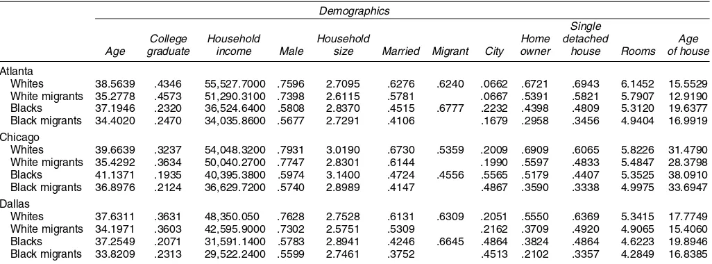
Table 1 provides some summary statistics concerning white and black migrants in our sample. In each city we com-pare migrants to all household heads who work, who are age 18–60, and who commute by car to work. A large share of the household heads move over a 5-year period. In Chicago, 54% of all whites and 46% of blacks switched homes between 1985 and 1990. Migrants are better educated but have lower household incomes than the entire population. Across the three cities, both black and white migrants are more likely to rent their home and to live in a smaller housing unit. In all three cities, black migrants are more likely to live in the suburbs than the average black household.
Table 1. Demographic Means for Migrants
Demographics
Single
College Household Household Home detached Age
Age graduate income Male size Married Migrant City owner house Rooms of house
Atlanta
Whites 38.5639 .4346 55,527.7000 .7596 2.7095 .6276 .6240 .0662 .6721 .6943 6.1452 15.5529 White migrants 35.2778 .4573 51,290.3100 .7398 2.6115 .5781 .0667 .5391 .5821 5.7907 12.9190 Blacks 37.1946 .2320 36,524.6400 .5808 2.8370 .4515 .6777 .2232 .4398 .4809 5.3120 19.6377 Black migrants 34.4020 .2470 34,035.8600 .5677 2.7291 .4106 .1679 .2958 .3456 4.9404 16.9919 Chicago
Whites 39.6639 .3237 54,048.3200 .7931 3.0190 .6730 .5359 .2009 .6909 .6065 5.8226 31.4790 White migrants 35.4292 .3634 50,040.2700 .7747 2.8301 .6144 .1990 .5597 .4833 5.4847 28.3798 Blacks 41.1371 .1935 40,395.3800 .5974 3.1400 .4724 .4556 .5565 .5179 .4407 5.3525 38.0910 Black migrants 36.8976 .2124 36,629.7200 .5740 2.8989 .4147 .4867 .3590 .3338 4.9975 33.6947 Dallas
Whites 37.6311 .3631 48,350.050 .7628 2.7528 .6131 .6309 .2051 .5550 .6369 5.3415 17.7749 White migrants 34.1971 .3603 42,595.9000 .7302 2.5751 .5309 .2162 .3709 .4920 4.9065 15.4060 Blacks 37.2549 .2071 31,591.1400 .5783 2.8941 .4246 .6645 .4864 .3824 .4864 4.6223 19.8946 Black migrants 33.8209 .2313 29,522.2400 .5599 2.7461 .3752 .4513 .2102 .3357 4.2849 16.8385
NOTE: The raw data are the 1990 U.S. Census of Population and Housing. This sample comprises all heads of households age 18–60 who work and who commute by car to work.
3. A MODEL OF HOUSING CHOICE
In this section we describe our model of housing demand. The model includesm=1, . . . ,M metropolitan areas. In each metropolitan area there are i=1, . . . ,Im individuals and j= 1, . . . ,Jm housing units. In what follows, we suppress m in much of our notation, because we treat each city as a separate market and do not pool data from across cities in our estimation. A home is a bundle of three types of attributes: physical at-tributes, community atat-tributes, and attributes observed by the consumer but not by the econometrician. The physical attributes include the number of rooms, the age of the unit, and dummy variables for ownership dummy and single detached dwelling. The community attributes in our model are the percentage of black households in the PUMA, the percentage of college-educated households in the PUMA, and whether the PUMA is located in the center city. We letxjdenote a 1×Kvector of the physical and community attributes of housing unitj, the unob-served product attribute is modeled as a scalarξj,and the price of the housing unit ispj.
Prices in the housing market are determined in equilibrium by the interaction of a large number of buyers and sellers. In the model, the price of housing unitjis a functionpm, which maps the characteristics of a housing unit into prices as follows:
pj=pm(xj, ξj). (1) Household utility is a function of housing characteristics(xj, ξj) and consumption of a composite commodityc, with a price nor-malized to $1 (pre-tax). The utility that consumerireceives for productj,uij,thus can be written as
uij=ui(xj, ξj,c). (2) We model the choice of housing as a static problem. As is well known, even if housing is durable, static first-order conditions will be appropriate if utility is time-separable,pm corresponds to the implicit rental value of housing, and there are no adjust-ment costs. The functionui should be interpreted as a house-hold’s utility from the flow of housing services, not its lifetime discounted utility.
Households are rational utility maximizers who choose their preferred bundle given their incomeyi. Productj∗(i)is utility maximizing for householdiif
j∗(i)=arg max j ui
xj, ξj,yi−pm(xj, ξj)
. (3)
Note that in (3) we have substituted the budget constraint di-rectly into the utility function.
Suppose that product characteristic k,xj,k, is a continuous variable and that productj∗ is utility maximizing for house-holdi. Then the following first-order condition must hold:
∂ui(xj∗, ξj∗,yi−pj∗) ∂xj,k
−∂ui(xj∗, ξj∗,yi−pj∗)
∂c
∂pm(xj∗, ξj∗) ∂xj,k
=0, (4)
∂ui(xj∗, ξj∗,yi−pj∗)/∂xj,k ∂ui(xj∗, ξj∗,yi−pj∗)/∂c =
∂pm(xj∗, ξj∗) ∂xj,k
. (5)
Equation (5) is the familiar condition that the marginal rate of substitution between a continuous characteristic and the com-posite commodity is equal to the partial derivative of the hedo-nic.
In the Census data only a single cross-section of households is observed. Obviously, we will not be able to learn an indi-vidual household’s entire utility function, ui, by observing it make only one choice. Some restrictions on the functionuiwill be required for identification (see Bajari and Benkard 2002). Therefore, we use the following specification for consumer preferences:
uij=βi,1log(roomj)+βi,2log(agej)+βi,3log(ξj)+βi,4ownj
+βi,5singlej+βi,6log(mblackj)
+βi,7log(mbaj)+βi,8cityj+c, (6) where
βi,k=fk(di)+ηi,k, (7)
E(ηi|di)=0. (8) In (6), the variables have the following interpretation:
• roomjis the number of rooms in housing unitj.
• agejis the age in years of housing unitj.
• ξj is the value of the characteristic seen to the consumer, but not by the economist, associated with housing unitj.
• ownj is a dichotomous variable equal to 1 if the housing unitjis owner occupied and 0 otherwise.
• singlejis a dichotomous variable equal to 1 if the housing unitjis detached and 0 otherwise.
• mblackj is the proportion of black heads of household in the PUMA where housing unitjis located.
• mbajis the proportion of college-educated heads of house-hold in the PUMA where housing unitjis located.
• cityj is a dichotomous variable equal to 1 if the housing unitjis located in the center city.
In the parametric model (6)–(8), each householdi’s utility is linear (or log-linear) in the various characteristics. However, we allow each household to have a unique set of taste parameters, βi,1−βi,8. Similar specifications for consumer utility are
com-monly made in the literature on demand estimation in differ-entiated product markets (see Berry et al. 1995; Petrin 2002). The termsβi are refered to as random coefficients. Random-coefficient models are considerably more flexible than standard logit or multinomial probit models, in which it is assumed that βi,k=βkfor alli; that is, the preference parameters are identical across households.
Modeling household preferences as a function of demo-graphics is common in the literature. In (7) and (8), theβi,k’s are modeled as a function,fk, of demographic characteristics,
di,and an orthogonal household-specific residual,ηi,k. In our application,di corresponds to the age of the head of house-hold, annual household income, household size, and dummy variables for whether the head of household is male, married, black, a college graduate, and a center city worker.
Our specification differs from previous work in two ways (see Berry et al. 1995; Petrin 2002). First, we do not include a random preference shock, such as an extreme value error term. Including this would not be appropriate in our work, because some product characteristics are modeled as continuous. Sec-ond, we do not make parametric assumptions about the distri-bution ofβi,korηi,kfor characteristicskthat are continous. In previous work, due to the computationally complexity of the estimators, theβi’s were often modeled as independent draws from a normal distribution. However, because of the compu-tational simplicity of our estimator, we do not need to impose such parametric assumptions.
If we make the functional form assumption (6), then (4) be-comes
βi,k
xj∗,k
=∂pm(xj∗, ξj∗)
∂xj,k
, (9)
βi,k=xj∗,k
∂pm(xj∗, ξj∗) ∂xj,k
. (10)
Equation (10) suggests that if we could recover an estimate of ∂pm(xj∗,ξj∗)
∂xj,k , then we could learn a household’s random coeffi-cient for characteristick,βi,k, by observingxj∗,k.In our micro data, we do in fact observe the housing characteristics chosen by each household. Using nonparametric methods, described in
the next section, we can flexibly estimate ∂pm(xj∗,ξj∗)
∂xj,k . There-fore, all of the terms on the right size of (10) can be recovered by the economist. This allows us to recover the unobserved, household-specific taste parameters,βi,k. This simple observa-tion, well understood in the hedonics literature, lies at the heart of our estimation strategy.
For product characteristics that take on dichotomous values of 0 or 1, there is no first-order condition for utility maximiza-tion. Instead, utility maximization implies a simple threshold decision making rule. For instance, suppose that household i
chooses product j∗. Definexi as a vector of observed char-acteristics with single=1 and all other elements set equal to their corresponding values in xj∗. Define xi similarly, ex-cept for single=0. The implicit price faced by household i
for single detached housing in the market is then pm single=
pm(xi, ξj)−pm(xi, ξj).Utility maximization implies that
[single=1] ⇒
βi,5>
pm single
, (11)
[single=0] ⇒
βi,5<
pm single
. (12)
That is, if householdilives in single detached housing, then we can infer thati’s preference parameter exceeds the implicit price for this characteristic. Analogous conditions can be derived for the other dichotomous characteristics.
4. ESTIMATION
Our estimation approach involves three steps. In the first step, we estimate the housing hedonic using flexible, nonparametric methods based on the techniques described by Fan and Gijbels (1996). In the second step, we use the first-order condition (10) to infer household-level preference parameters for continuous product characteristics. In the third step, we estimate (7) and (8) by regressing household-level preference parameters on the de-mographic characteristicsdi. We also discuss how to estimate preferences for dichotomous characteristics by maximum like-lihood.
4.1 First Step: Estimating the Hedonic
We have experimented with several different methods for estimating the hedonic, including high-order polynomials and kernel regression. The method that produced the most appeal-ing estimates are based on local polynomial modelappeal-ing. To es-timate the implicit prices faced by household i, who chooses
j∗(i), we suppose that locally, the hedonic satisfies
pj=α0,j∗+α1,j∗log(roomj)+α2,j∗log(agej)
+α3,j∗ownj+α4,j∗singlej+α5,j∗log(mblackj)
+α6,j∗log(mbaj)+α7,j∗cityj+ξj.
In our notation we denote the hedonic coefficients byα0,j∗− α7,j∗ to emphasize the fact that our estimates are local in the sense that a unique set of implicit prices is estimated for each value ofj=1, . . . ,Jm in marketm.The error term to the he-donic is interpreted asξj, a vertical product characteristic ob-served by the consumer, not by the economist. Following Fan
and Gijbels (1996), we use weighted least squares to estimate trix of regressors, which for each product includes an intercept and seven characteristics; andWis aJm×Jmmatrix of kernel weights. Notice that in our analysis we do not pool observa-tions across markets m. The hedonic is meant to capture the budget constraint faced by consumeri. Because different mar-kets may be in different equilibria, pooling data would not be appropriate. Also, notice that the kernel weights are a function of the distance between the characteristics of productj∗ and productj. Thus the local linear regression assigns greater im-portance to observations with characteristics close toj∗. Local linear methods have the same asymptotic variance and a lower asymptotic bias than the Nadaraya–Watson estimator. Also, the Gasser–Mueller estimator has the same asymptotic bias and a higher asymptotic variance than local linear methods.
Our estimates of (13) and (14) allow us to recover an estimate of the unobserved product characteristic,
ξj∗=pj∗−
In (15), the unobserved product characteristicξj∗is estimated as the residual to our hedonic regression. Although there certainly are other interpretations of the hedonic residual, we believe that this interpretation is the most important in our data. Given the lack of appropriate instruments, we maintain the standard hedo-nic assumption that the unobserved product characteristics are independent of the observed product characteristics.
In local linear regressions, the choice of kernel and band-width is extremely important. We chose the following normal kernel function with a bandwidth of 3:
K(z)= In (16) the functionKis a product of standard normal distribu-tions, which we denote byN. In equation (16), for thekth char-acteristic, we evaluate the normal distribution atzk/σk2,where
σk2is the sample standard deviation of characteristick. Fan and Gijbels (1996) described asymptotically appropriate methods for choosing the bandwidth. However, in our application, be-cause the hedonics depend on seven covariates, these methods are not likely to be very reliable, due to the curse of dimension-ality. Based on visual inspection of the estimates, we choose the bandwidth equal to 3.
Given the large number of covariates, we should not interpret these estimates as “nonparametric.” However, compared with other flexible functional forms, local linear methods appeared to give much more plausible estimates of the implicit prices. In all three cities, the estimated implicit prices have intuitively plausible signs and magnitudes.
4.2 Second Step: Applying the First-Order Conditions
After estimating the implicit prices, we next estimate the preferences for continuous characteristics. If household i
chooses productj∗, then (10) must hold. Using estimates of implicit prices obtained from the first step and the observed choice ofxj∗,k, an estimationβi,k ofβi,k can be recovered as
In (18) we recover householdi’s preference for characteristick
using our estimate of the (local) implicit price recovered from the first step,∂pm(xj∗,ξj∗)
∂xj,k .Because we observe each household’s choice,xj∗,k, we can recover an estimate of the unobserved taste parameter,βi,k.
Because the preference parameter for every individual can be recovered using our first-order condition, the population distrib-ution of tastes in marketmcan also be estimated. If we observed a sufficiently large number of households, then we could non-parametrically recover the joint distribution of theβi,k for the continuous product characteristics. Therefore, we can identify a nonparametric distribution of these random coefficients (see Bajari and Benkard 2002 for more discussion). In the next step we describe how to estimate the joint distribution of tastes and demographics.
4.3 Third Step: Modeling the Joint Distribution of Tastes and Demographics
After recovering household-level preference parameters, we then estimate (7) and (8). We could easily do this using very flexible local linear methods. However, for presentation pur-poses, it is more convenient to model the joint distribution of tastes and demographic characteristics using a linear model. For continuous characteristics, we let
βi,k=θ0,k+
s
θk,sdi,s+ηi,k. (19)
We then simply estimate (19) using regression. The regression that we run is
In (20) we have simply substituted our estimate ofβi,kfrom the second stage into (19).
Given estimates θk,s, the residuals can be interpreted as household-specific taste shocks. Note that, once again, we have not imposed any parametric restrictions on theηi,k. Previous work, such as that of Berry et al. (1995) and Petrin (2002) im-posed parametric assumptions on taste shocks because of the computational demands of their estimators. Because our esti-mator is computationally light, such requirements are not nec-essary.
Equations (11) and (12) imply that preference parameters for dichotomous characteristics are not identified. We can only in-fer that the prein-ferences for a particular household are above or below the threshhold value equal to the implicit price of the discrete characteristic. Given this lack of identification, we use a parametric model for these taste coefficients. We assume, as
in (19), that preferences are linear functions of demographics. However, unlike in the continuous case, we impose a paramet-ric distribution onηi,k. For this application, we assume that they are normally distributed, although other distributions could also be easily estimated. Ifηi,k is normally distributed with mean 0 and standard deviationσ, then, by (11) and (12), the probabil-ity that householdi=1, . . . ,Ichooses to live in single detached
whereNis the normal cdf. The likelihood function for the pop-ulation distribution of tastes for single detached housing can be written as householdipurchases single detached housing and 0 otherwise. This is a version of the probit model where instead of normal-izingσ=1, we have normalized the coefficient on price equal to−1. We estimate this model using maximum likelihood.
In principal, we could model correlation between the taste coefficients for all discrete product characteristics using a mul-tivariate normal distribution and estimate a more flexible model of how tastes for characteristics are correlated. However, for ex-positional clarity, we estimate the tastes for each product char-acteristic independently. An alternative approach, which does not require assuming that tastes lie in a parametric family, is to use the bounds approach described by Bajari and Benkard (2002).
4.4 Discussion
Because the methods that we use are somewhat unique, it is useful to compare our approach with methods that have been used to estimate the demand for housing attributes and the demand for differentiated products more generally. First, the recent literature on estimating discrete choice models has emphasized that price elasticities tend to be biased toward 0 if the economist fails to account for ξj, product characteris-tics observed by the consumer but not by the economist (see, e.g., Berry 1994; Berry et al. 1995; Petrin 2002; Ackerberg and Rysman 2002). This problem is ignored in most previous stud-ies of housing demand with the exception of the study of Bayer et al. (2002). We expect this problem to be especially important in housing research based on standard Census data, where re-searchers commonly find that the observed covariates explain only one-half or less of the variation in prices.
Second, our model allows for a flexible specification of the joint distribution of tastes and demographic characteristics. In
our model we estimate the distribution of eight random coeffi-cients (seven for the observed product characteristics and one for the unobserved product characteristic) as a function of eight demographic variables. Parametric assumptions about the dis-tribution of random coefficients are not imposed during esti-mation. In most previous work that estimated discrete choice models (e.g., Berry et al. 1995; McCulloch et al. 2000), the random coefficients are typically assumed to be independently and normally distributed, conditional on demographics. Given that these models are computationally intensive, such parsimo-nious parametric specifications are required to make the prob-lem computationally feasible. In contrast, our procedure is easy to compute and can be quickly estimated using standard statis-tical packages.
The analyst does face a couple of trade-offs, however, in us-ing our approach as compared with the random coefficient logit model estimated by Berry et al. (1995) or the random coef-ficient probit estimated by McCulloch et al. (2000). The first such trade-off is that in characteristic models such as ours, not all products are strong gross substitutes. The number of prod-ucts with positive cross-price elasticities is proportional to the number of characteristics used in the analysis (see Anderson, DePalma, and Thisse 1995 for a complete discussion). In our example, because there are eight product characteristics, we do not believe that this is particularly problematic; however, it can be an issue in datasets with fewer product characteristics. Second, the instrumental variable strategies proposed by Berry et al. (1995) cannot be implemented in our model in a straight-forward fashion.
Third, although our approach to estimating preferences is similar to the hedonic two-step of Rosen (1974) and Epple (1987), there are some important distinctions. In our model, household-level preferences are only locally identified from a single cross-section of data. Although we do regress prefer-ences on household-level demographics to obtain an estimate of how preferences change with demographic characteristics of the household, we do not attempt to globally estimate prefer-ences as in the standard second-stage hedonic regression. As a result, our procedure does not involve a step requiring the economist to regress product characteristics on nonlinear func-tions of product characteristics, which has been criticized as a limitation of the second stage (Brown and Rosen 1982). Epple (1987) presented a formal model of the necessary conditions for achieving identification of structural parameters using the hedonic two-step. Finding valid instruments to implement this procedure is often quite challenging. Hedonic researchers have instead attempted alternative identification strategies, such as pooling multiple segmented markets at a point in time and argu-ing that differences in equilibrium prices and quantities across markets reflect differences in supply conditions, and this varia-tion traces out “the” demand curve (Palmquist 1984).
Our article is most closely related to the important recent contributions of Epple and Sieg (1999) and Bayer et al. (2002). Like Epple and Sieg (1999), we seek to estimate the demand for local pubic goods. Unlike their approach, we work with micro data that provide demographic information on who lives in each housing unit and housing and community attributes. Using our micro data, we choose to focus solely on recent migrants’ hous-ing choices. Thus we are able to trace out their heterogenous
tastes for different demographic groups and to study how dif-ferences in place of work affect residential choice. By estimat-ing our model solely for migrants, we avoid the problem that in any cross-section, some households are living in their “fa-vorite” affordable housing product, whereas other households would relocate if transaction costs were zero but due to positive transaction costs (selling a home, moving one’s possessions) they are “stuck.” Assuming that migrants are not a select sample of the population, migrant housing choice is more informative about preferences over housing attributes.
A limitation of our approach compared with the research of Epple and Seig (1999) and Bayer et al. (2002), however, is that we do not present an equilibrium model of the entire hous-ing market that could be used to compute interesthous-ing policy counterfactuals. Bayer et al. (2002) applied techniques similar to those of Berry et al. (1995) to estimate a model of hous-ing demand ushous-ing a rich dataset from the San Francisco Bay area. However, it is worth noting that the magnitudes of our hedonic estimates are roughly consistent with the hedonic re-gressions that Bayer et al. presented. In particular, like Bayer et al., we find that the implicit price for increasing the fraction of college-educated residents is several times larger than that for increasing the percentage of white residents. As a result, hedonic methods would lead to the conclusion that there is a much greater willingness to pay for the educational status of one’s neighbors than the race of one’s neighbors. This conclu-sion results from simple revealed preference logic: goods that are priced higher are more highly valued at the margin with all else held constant. This conclusion will hold whether micro community data are used (as in Bayer et al. 2002) or a more aggregated definition of a community is used as in our analysis. We view the lack of micro community data as a limitation of our analysis compared to that of Bayer et al. On the other hand, unlike Bayer et al., we conduct our analysis on multiple cities instead of a single city, and our analysis allows for nonparamet-ric random coefficients.
Finally, one appealing feature of our analysis is that it is very transparent. Hedonics is a well-understood and popular tech-nique in housing research. It makes clear, using simple econo-metric methods, exactly what needs to be assumed about the joint distribution of observed and unobserved product charac-teristics to correctly calculate the implicit prices. Then, from the hedonics, we simply use the implicit prices to engage in revealed preference.
There are at least four limitations to the model of housing demand presented in the previous section. The first limitation is the standard exogeneity assumptions used in hedonics. In gen-eral, one would not expect unobserved product characteristics to be independent of observed product characteristics. In our opinion, bias in implicit prices is primarily a data issue. With sufficiently detailed data, one can recover plausible estimates of implicit prices. However, to the best of our knowledge, there are no publicly available data sources in which we can merge the detailed demographic data used in the Census with detailed data on home prices and characteristics. To address this prob-lem, we checked our estimates of implicit prices against those found by other researchers to make sure that they appeared rea-sonable. This problem is not unique to hedonics; most discrete choice models similarly assume that product characteristics are exogenous.
Second, in estimating the first-stage hedonic, we face the concern that PUMAs are too big to yield credible first-stage im-plicit prices. In estimating the first-stage hedonic regressions, we merge into each individual home price data the characteris-tics of the PUMA where the home is located. The characterischaracteris-tics that we use are the percentage of PUMA’s population who are black, the percentage of PUMA’s who are college graduates, and whether the PUMA is located in the metropolitan area’s central city. Fortunately, our recent work using real estate data from the year 2002 in Los Angeles County suggests that he-donic estimates of implicit prices are quite robust to whether they are estimated using “micro” Census block information or more “macro” zip code information. We are able to show this because our proprietary dataset from First American Real Es-tate Solutions provides sales price data, home characteristics and the home’s Census block, Census tract, and zip code. For these three different levels of geography, we find quite compa-rable implicit prices for the “community’s” percent blacks and percent college graduates. We believe this indicates that there is significant positive spatial correlation in these attributes. Pre-vious hedonic research using PUMAs as the community indi-cator has generated credible hedonic estimates. DiPasquale and Kahn’s (1999) hedonic study of Los Angeles County estimated micro hedonic home price regressions. Using PUMA-level ge-ographic identifiers, these authors reported a plausible set of implicit price estimates for a range of local public goods.
Third, the results of our analysis will depend to some ex-tent on the functional form of the utility function. Given that we have only a single cross-section of data, it is not possible to globally identify preferences. We note, however, that we impose the minimal functional form assumptions required for identifi-cation. Also, many of the results that we present are based on the willingness to pay for fairly small changes in the bundle consumed by a household. Because the marginal rate of substi-tution for continuous characteristics is identified without func-tional form assumptions, many of our results will remain robust for a large set of alternative specifications for preferences.
Fourth, we recognize that observed differences in mean will-ingness to pay for housing attributes between whites and blacks may represent factors other than preferences. Although we con-trol for household head educational attainment and household income, race may still proxy for permanent income and wealth accumulation (see Duca and Rosenthal 1994; Charles and Hurst 2002). Despite the limitations of this exercise, we believe that flexibly modeling the joint distribution of tastes and demo-graphic characteristics is an important step toward better un-derstanding the determinants of housing demand.
5. RESULTS
This section presents estimates of the model for three cities to test three hypotheses for why whites choose suburban hous-ing products while blacks tend to choose center city houshous-ing products. The first hypothesis is that whites and blacks have different demands for the physical attributes of housing. Sub-urban homes are larger, newer, and more likely to be single detached, owner-occupied units relative to center city housing units. Blacks may have a lower demand for such products be-cause their household incomes are lower than whites. The sec-ond hypothesis is that racial segregation is inextricably tied to
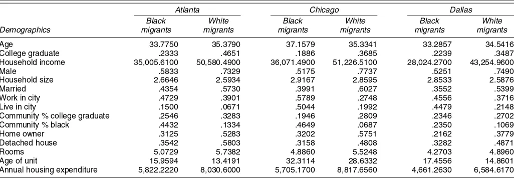
Table 2. Summary Statistics for the Migrants Included in the Structural Estimation
Atlanta Chicago Dallas
Black White Black White Black White
Demographics migrants migrants migrants migrants migrants migrants
Age 33.7750 35.3790 37.1579 35.3341 33.2857 34.5416 College graduate .2333 .4651 .1886 .3685 .2239 .3487 Household income 35,005.6100 50,580.4900 36,071.4900 51,226.5100 28,024.2700 43,254.9600 Male .5833 .7329 .5175 .7737 .5251 .7490 Household size 2.6646 2.5934 2.9167 2.8595 2.8533 2.5876 Married .4354 .5730 .3991 .6027 .3552 .5399 Work in city .4729 .3901 .5789 .2748 .4556 .3716 Live in city .1500 .0671 .5044 .1992 .4479 .2148 Community % college graduate .2546 .3283 .1946 .2809 .2346 .2702 Community % black .4432 .1334 .4649 .0687 .2350 .1069 Home owner .3125 .5283 .3202 .5751 .2162 .3779 Detached house .3542 .5803 .3158 .4808 .3282 .4871 Rooms 5.0729 5.7382 4.8860 5.5248 4.2703 4.8960 Age of unit 15.9594 13.4191 32.3114 28.6332 17.4556 14.8601 Annual housing expenditure 5,822.2220 8,030.6000 5,705.1700 8,817.6560 4,661.2630 6,584.6170
NOTE: This table reports sample means for 2,000 observations for each city drawn at random from the set of migrants.
local labor markets and the disutility from commuting. If mi-nority employment is disproportionately located in center cities and if the disutility from commuting is high, then blacks will urbanize. The third hypothesis focuses on peer group selec-tion. Communities differ with respect to their racial composi-tion and human capital levels. A household will recognize that by choosing a particular community, they will determine who will be their neighbors and who their children will go to school with. The average suburban community has more college grad-uates and fewer minorities than the average urban community. Blacks and whites may differ with respect to their willingness to pay for these attributes. We recognize that another hypothesis is that black households seeking suburban housing products are discriminated against (Yinger 1986; Munnell, Tootell, Browne, and McEneaney 1996). Detecting and accounting for perceived or actual discrimination is beyond the scope of this article (see Heckman 1998).
To ease the computational burdens in estimating the flexi-ble hedonic specification, we drew a random sample of 2,000 migrants for each city. These three samples of 2,000 observa-tions each will form the basis for all of our subsequent empirical work. Table 2 presents the sample demographic means for white and black migrants included in our structural estimates across the three metropolitan areas. Across the three cities, the age white household’s income is $15,000 higher than the aver-age black household’s. White household heads are much more likely to be married than black household heads. This marriage differential is 14 percentage points in Atlanta, 20 percentage points in Chicago, and 17 percentage points in Dallas. Aver-aged across the three cities, white household heads are 18 per-centage points more likely to be a college graduate than black household heads.
5.1 Hypothesis 1: The Demand for Physical Housing Attributes and Housing Type
The suburban housing stock features homes that are larger, newer, and more likely to be single detached relative to the cen-ter city housing stock. The standard explanation for this fact is that the housing stock is durable and land’s price per square
foot falls with distance from the central business district to com-pensate for the longer commute downtown (Alonso 1964). We test whether whites and blacks have different tastes for such at-tributes and whether average demographic differences between races such as differences in income, educational attainment, and marriage rates explain differences in the demand for physical attributes of the housing unit.
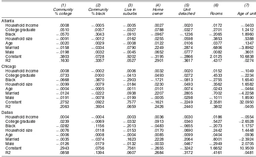
Reduced-form evidence documents the differences in hous-ing consumption across demographic groups for the migrant samples. Table 3 presents ordinary least squares regression re-sults from 21 separate regressions. In each regression we con-trol for the household income and household size and for the household head’s education, race, age, sex, and marital status. Column (6) reports the regression where the dependent variable is the housing unit’s number of rooms. We find that married households live in homes that have .68 more rooms in Atlanta and .7 more rooms in Chicago than nonmarried households. Across the three cities, married migrants are more than 20 per-centage points more likely to own a home and to live in a single detached suburban home. An extra $10,000 in household in-come increases the propensity to own a home by 3 percentage points in each of the cities.
For each city, we estimate the structural model presented in Section 3. This yields for each housing attribute, a preference parameter for each migrant. The discrete choice literature has modeled such random coefficients as normally distributed. Fig-ure 1 presents a histogram of the taste parameters for rooms for the 2,000 Chicago migrants. The important point conveyed by this figure is that tastes are right-skewed and are not nor-mally distributed. Preferences across housing attributes are not independently distributed. Table 4 reports, by city, the correla-tion matrix of tastes across attributes. Across all three cities, the taste for rooms and the taste for communities with high levels of human capital are positively correlated. Surprisingly, the taste for communities with high levels of minorities is positively cor-related with the taste for high human capital communities.
To test hypothesis 1, we use the random coefficient estimates to construct willingness to pay for an increase in rooms from 4 to 6. LetWTPROOMSidenote householdi’s willingness to pay to increase the number of rooms from 4 to 6. By (6), this must
Table 3. Descriptive Ordinary Least Squares Regressions of Migrant Housing Choice
(1) (2) (3) (4) (5) (6) (7)
Community Community Live in Home Unit
% college % black suburbs owner detached Rooms Age of unit
Atlanta
Household income .0008 −.0005 −.0005 .0027 .0020 .0172 −.0403 College graduate .0510 .0057 −.0327 .0788 .0327 .2701 1.2412 Black −.0570 .3043 −.0910 −.0967 −.1236 −.2065 1.8960 Household size −.0091 −.0012 .0162 .0255 .0598 .3853 .5388 Age −.0020 .0029 −.0008 .0122 .0106 .0377 .1347 Married −.0158 −.0334 .0790 .2249 .2874 .6806 −3.8962 Male −.0198 .0032 −.0045 .0652 .0777 .0082 .3601 Constant .3803 .0728 .9202 −.3195 −.2866 2.0125 10.6838 R2 .1630 .3357 .0527 .2901 .3617 .4317 .0274 Chicago
Household income .0008 −.0002 .0006 .0032 .0020 .0152 −.1049 College graduate .0733 .0000 −.0413 .0493 .0272 .4533 −.2234 Black −.0668 .3870 −.2903 −.1721 −.0813 −.2755 1.6540 Household size −.0099 .0079 −.0184 .0230 .0493 .3562 1.6582 Age −.0004 −.0005 .0011 .0101 .0074 .0243 −.0464 Married −.0124 −.0222 .0938 .2207 .2805 .7002 −4.2258 Male −.0191 −.0078 −.0199 −.0005 .0298 −.1011 1.8590 Constant .2752 .0922 .7577 −.1621 −.2249 2.3581 32.0950 R2 .2063 .3934 .0659 .2426 .2440 .3802 .0405 Dallas
Household income .0004 −.0004 .0003 .0036 .0030 .0186 −.0554 College graduate .0239 −.0069 −.0332 .0913 .0340 .5427 −2.6528 Black −.0282 .1156 −.2013 −.0483 −.0655 −.2073 1.1757 Household size −.0076 .0118 −.0153 .0170 .0690 .2442 1.4448 Age −.0006 .0008 −.0004 .0085 .0099 .0404 .0936 Married −.0035 −.0374 .1623 .2228 .2064 .8001 −2.3924 Male −.0126 .0179 −.0132 −.0033 .0467 −.2949 2.0705 Constant .2943 .0756 .7561 −.2655 −.3242 1.6652 10.9509 R2 .0858 .1394 .0607 .2684 .3172 .4161 .0481
NOTE: This table reports 21 reduced-form ordinary least squares regressions, 7 for each city. The dependent variables “live in suburbs,” “home owner,” and “unit detached” are dummy variables. In each regression, housing consumption measures are fitted as a function of personal attributes. The omitted category is a white, noncollege graduate who is female and not married. Household income is measured in thousands of 1989 dollars. There are 2,000 observations in each regression.
satisfy
WTPROOMSi=β1,i
log(6)−log(4). (24)
This measure of willingness to pay for structure is regressed on household demographics. Table 5 reports these estimates of willingness to pay for two more rooms for each of the three cities. Across all three cities, richer, college-educated, married migrants in larger households are willing to pay more for more space. Holding all of these demographics constant, blacks are
Figure 1. Chicago Migrant Preference Heterogeneity Over Housing Unit Size.
willing to pay $399 per year less in Chicago for the extra living space. In Atlanta, all else being equal, blacks are willing to pay $172 less for extra living space.
But all else is not equal. As shown in Table 2, blacks have lower incomes, lower college-graduate rates, and lower mar-riage rates. Based on the Atlanta coefficient estimates, if blacks caught up to the average white levels for these three demo-graphic categories, then their willingness to pay for rooms would significantly increase. Demographic differences matter as much as “taste differences” in explaining the demand for physical attributes across races. The differential demand for housing unit size between whites and blacks is our strongest
Table 4. Correlation Matrix of Marginal Utilities by Metropolitan Area
Community
Rooms Age of unit % BA
Atlanta
Age of unit .0749
Community % BA .1347 −.0475
Community % black .0219 .2264 .4577 Chicago
Age of unit .1231
Community % BA .4126 .1783
Community % black .1259 .1414 .3687 Dallas
Age of unit .0414
Community % BA .2501 .1458
Community % black .1476 .2561 .4633
Table 5. Estimates of the Willingness to Pay for Rooms
Demographics Atlanta Chicago Dallas
Age 21.9402 19.4257 22.8256 (2.3616) (2.7855) (2.0161) College graduate 184.7462 378.0459 316.2760
(41.5490) (55.0933) (40.9990) Black −172.3309 −398.7179 −140.3617
(44.1881) (67.9734) (55.7413) Household income 10.2370 12.4079 11.0030
(.8263) (1.0465) (.6090) Household size 209.7445 217.7264 132.4001
(17.9231) (28.7072) (14.8875) Male 30.3560 −53.2453 −149.3462
(47.5370) (59.4864) (47.9940)
NOTE: Each column of the table presents a separate ordinary least squares regression. The dependent variable is a migrant’s willingness to pay per year for an increase from four to six rooms in a housing unit, holding all other housing product attributes constant. Standard errors are reported in parentheses. The omitted category is a white, noncollege graduate who is female and not married. Household income is measured in thousands of 1989 dollars.
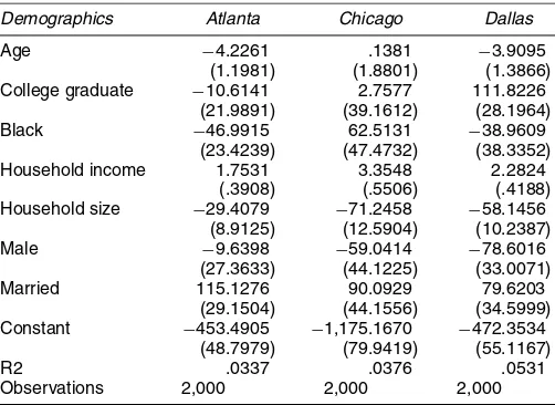
housing structure evidence for why black urbanization takes place. For other physical attributes of housing, we do not find such major differences in willingness to pay between groups. Table 6 presents our estimates for how much migrants are will-ing to pay to live in a house that is 35 years old versus a house that is 10 years old. Across all three cities, migrants are will-ing to pay for newer houswill-ing, but the differences in willwill-ingness to pay across demographic groups are small. For example, in Chicago a college graduate is willing to pay $2.76 more than an identical non–college graduate to live in older housing.
Table 7 presents estimates of the household willingness to pay to own based on (22). Note that the price coefficient has been normalized to equal −1. In Chicago, the college-educated are willing to pay $72 more per year. An extra $10,000 in household income increases willingness to pay to own by $44 per year. Only in Atlanta do we reject the hypothesis that
Table 6. Estimates of the Willingness to Pay for an Older Housing Unit
Demographics Atlanta Chicago Dallas
Age −4.2261 .1381 −3.9095 (1.1981) (1.8801) (1.3866) College graduate −10.6141 2.7577 111.8226
(21.9891) (39.1612) (28.1964) Black −46.9915 62.5131 −38.9609
(23.4239) (47.4732) (38.3352) Household income 1.7531 3.3548 2.2824
(.3908) (.5506) (.4188) Household size −29.4079 −71.2458 −58.1456
(8.9125) (12.5904) (10.2387) Male −9.6398 −59.0414 −78.6016
(27.3633) (44.1225) (33.0071) Married 115.1276 90.0929 79.6203
(29.1504) (44.1556) (34.5999) Constant −453.4905 −1,175.1670 −472.3534
(48.7979) (79.9419) (55.1167) R2 .0337 .0376 .0531 Observations 2,000 2,000 2,000
NOTE: Each column of the table presents a separate ordinary least squares regression. The dependent variable is a migrant’s willingness to pay per year for an increase from 10 to 35 years in the age of a housing unit, holding all other housing product attributes constant. Standard errors are reported in parentheses. The omitted category is a white, noncollege graduate who is female and not married. Household Income is measured in thousands of 1989 dollars.
Table 7. Probit Estimates of the Demand for Owning
Demographics Atlanta Chicago Dallas
Age 5.7628 10.8808 .9960 (.5457) (1.4349) (.1411) College graduate 53.5150 72.3841 13.0556
(9.8024) (28.3355) (2.8978) Black −38.1048 −48.5070 5.2907
(10.6864) (39.3679) (4.0455) Household income 1.5823 4.4116 .3716
(.1747) (.5000) (.0450) Household size 18.6377 50.4153 4.8466
(4.1044) (8.8029) (1.0871) Male 25.6344 12.8634 −2.1273
(11.0205) (31.8090) (3.5123) Married 64.2837 165.0626 8.5168
(11.8269) (30.9482) (3.6587) Price of ownership −1.0000 −1.0000 −1.0000 Constant −315.7914 −301.8911 52.2557 (22.9383) (62.5935) (6.1095) Pseudo-R2 .4105 .4240 .6889 observations 2,000 2,000 2,000
NOTE: Each column of the table presents a separate probit estimate. The dependent variable is a dummy variable that equals 1 if the migrant owns a home and 0 otherwise, holding all other housing product attributes constant. Standard errors are reported in parentheses. The omitted category is a white, noncollege graduate who is female and not married. Household Income is measured in thousands of 1989 dollars.
whites and blacks have equal willingness to pay to own. It is important to note that with our one cross-section of data, we are estimating a static model of housing demand. We recognize that the tenure choice decision has a dynamic component.
Table 8 presents the willingness to pay differentials for single detached housing. In Atlanta and Chicago, blacks are willing to pay less for such housing. In Chicago, all else being equal, blacks are willing to pay $410 less per year for such housing than whites. Similar to the case of rooms, married people are willing to pay more to live in single detached housing. Because blacks have lower marriage rates, this contributes to the total white–black gap with respect to demand for physical attributes. Although household income and educational attainment sharply
Table 8. Probit Estimates of the Demand for Single Detached Housing
Demographics Atlanta Chicago Dallas
Age −.0211 16.1145 .1754 (.4314) (2.5122) (.2191) College graduate −.6411 82.1002 −6.5952
(7.3269) (49.7589) (4.4498) Black −36.5337 −409.6949 −5.5963
(7.2683) (76.1423) (5.7880) Household income .3890 5.9420 .0345
(.1682) (.7282) (.0850) Household size 3.7795 75.1032 −.2434
(2.9635) (15.7585) (1.3193) Male −6.0654 31.6040 3.2634
(8.0832) (61.4414) (5.0320) Married 40.8022 598.1848 10.2411
(9.3722) (57.0570) (4.7934) Price of single detached unit −1.0000 −1.0000 −1.0000 Constant 236.9936 −815.7973 −23.6736 (25.4464) (127.1599) (9.8171) Pseudo-R2 .9343 .2369 .9170 Observations 2,000 2,000 2,000
NOTE: Each column of the table presents a separate probit estimate. The dependent variable is a dummy variable that equals 1 if the migrant lives in a detached home and 0 otherwise, hold-ing all other houshold-ing product attributes constant. Standard errors are reported in parentheses. The omitted category is a white, noncollege graduate who is female and not married. Household income is measured in thousands of 1989 dollars.
increase demand for detached housing in Chicago, such income effects have a much smaller impact in Atlanta and Dallas.
5.2 Hypothesis 2: Commuting and Place of Work
Employment suburbanization has tracked residential subur-banization for the last 50 years in the United States (Garreau 1992; Glaeser and Kahn 2001). As workers have suburbanized, many jobs have followed them to the suburbs. As jobs migrate to the suburbs, suburban residents have shorter commutes, and land-intensive firms can purchase more land cheaper than in the central business district. Atlanta, Chicago, and Dallas all have a significant amount of employment located outside of their cen-ter cities.
Such “job sprawl” could increase the black/white suburban-ization gap if households do not like commuting and blacks tend to work in highly urbanized industries. In our migrant At-lanta sample, 59% of workers work in the suburbs and 53% of black workers work in the suburbs. In Chicago, 70% of work-ers work in the suburbs and 42% of black workwork-ers work in the suburbs. In Dallas, 62% work in the suburbs and 54% of blacks work in the suburbs.
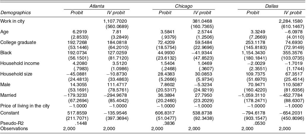
The commuting hypothesis posits that blacks live in the city because they work in the city. We test this hypothesis in Ta-ble 9 by estimating the demand for living in the city, as in (22). For each of the three cities, we estimate two separate models. We first estimate how much blacks are willing to pay to live in the city, holding all other migrant demographics and housing choice attributes constant. In Atlanta and Dallas, all else being equal, blacks are willing to pay $192 and $1,154 a year more than whites to live in the city. To test how much of this black differential willingness to pay is driven by place of work, we in-clude in the specification a dummy variable indicating whether the migrant works in the center city. We recognize that working
in the city is an endogenous regressor. Migrants may work in the city because they found out about a job opportunity from a city neighbor. In a job search model, living in the city raises one’s probability of working in the city.
We seek an instrumental variable for the place of work dummy variable. A valid instrument raises the probability of working in the center city and is unrelated to the place of residence decision. Labor economists have documented that workers develop industry-specific human capital (Neal 1995). Urban economists have established that industries differ with respect to their agglomeration rates in center cities versus sub-urbs. Land-intensive industries are less likely to urbanize and more likely to agglomerate at the suburban fringe. Glaeser and Kahn (2001) showed that manufacturing industries suburban-ize, whereas high human capital–intensive industries are more likely to locate within the center city. This suggests that a worker’s industry may be a valid instrument for place of work. Workers who have made an irreversible investment in industry-specific human capital in an industry that is disproportionately located in the center city have an incentive to work in the center city. We thus instrument for whether a migrant works in the city using the worker’s industry information (dummy variables for whether the migrant works in manufacturing, wholesale, retail, services, construction, or government).
For each city, we present our results where we include the work in city indicator and instrument for this variable. In all three cities, including this variable sharply reduces black will-ingness to pay to urbanize. In Dallas, black willwill-ingness to pay falls from $1,154 to $355 when place of work is controlled for and in Chicago the hypothesis that the black coefficient is 0 cannot be rejected. It is important to note that the first-stage in-strumental variable results have anR2of .02 for each city. Still, across the three cities, we find that black employment urbaniza-tion helps explain black residential urbanizaurbaniza-tion.
Table 9. Probit Estimates of the Demand for Living in the Center City
Atlanta Chicago Dallas
Demographics Probit IV probit Probit IV probit Probit IV probit
Work in city 1,107.7020 381.0468 2,284.1580 (560.0689) (160.7365) (610.1467) Age 6.2919 7.81 3.5841 2.5744 3.3249 −6.0978
(2.8533) (3.2849) (.9379) (1.2506) (7.2669) (4.0110) College graduate 192.7268 184.0818 72.4209 59.5484 253.1178 74.6930
(53.1446) (64.2010) (18.5754) (22.9696) (145.8183) (72.9149) Black 192.0734 127.0259 44.9930 −41.9344 1,154.3430 355.3576
(56.1501) (81.7120) (23.6132) (47.8523) (180.1841) (103.0735) Household income 4.2080 3.5120 1.5404 1.0469 −2.0029 −1.7019
(.7983) (1.0986) (.2468) (.3607) (2.3551) (1.1744) Household size −45.0881 −10.8730 28.4383 30.0853 109.7375 67.3517
(24.4813) (33.4863) (5.2666) (5.9734) (51.6970) (25.4514) Male 14.3055 111.4717 7.8602 −5.3234 70.9471 110.5087
(53.1691) (78.5761) (20.5317) (24.9219) (160.4220) (81.6356) Married −179.3233 −294.9678 36.3894 27.7950 −1,059.3110 −452.7784
(67.2694) (85.4042) (20.2460) (23.2029) (178.2471) (88.6307) Price of living in the city −1.0000 −1.0000 −1.0000 −1.0000 −1.0000 −1.0000 Constant 517.8559 −135.9546 606.8317 538.8738 −794.6178 −654.2031 (211.7071) (397.3694) (51.0477) (92.3438) (903.1547) (450.8096) Pseudo-R2 .1448 .3836 .0530
Observations 2,000 2,000 2,000 2,000 2,000 2,000
NOTE: Each column of the table presents a separate probit estimate. The dependent variable is a dummy variable that equals 1 if the migrant lives in the city and 0 otherwise, holding all other housing product attributes constant. Standard errors are reported in parentheses. IV probit indicates that the probit was estimated using an instrumental variables strategy. The dummy variable “work in city” equals 1 if a migrants works in the city. This variable is instrumented for using dummy variables for what industry the migrant works in. The omitted category is a white, noncollege graduate who is female, is not married, and works in the suburbs. Household income is measured in thousands of 1989 dollars.
Our structural estimates provide some insights into migrant value of time. This is relevant for judging the plausibility of our parameter estimates. Chicago migrants who work in the city are willing to pay $381 more per year to live in the city than are mi-grants who work in the suburbs. Mimi-grants who commute by car and work and live in city have an 11-minute-shorter one-way commute than migrants who live in the city and work in the suburbs. This suggests that migrants are willing to pay $4.15 to avoid an hour of commuting. Many travel cost studies as-sume that people value their commute time at 50% of their hourly wage; our Chicago estimate is roughly in line with this assumption.
5.3 Hypothesis 3: The Demand for Peers
Each day we interact with our neighbors. Thus their attributes affect our well-being and our human capital accumulation. He-donic studies have measured the benefit of having high-skilled neighbors by studying land rents in high- and low-skill areas (Rauch 1993; DiPasquale and Kahn 1999). Other empirical studies have measured peer group effects by regressing out-come measures, such as a person’s employment status, on the average of this outcome measure for one’s peer group (Case and Katz 1991; Crane 1991). The practical problem of measur-ing social externalities associated with peer exposure has led to an econometrics literature focused on the reflection prob-lem (Manski 1993). An alternative to the “production function” method for recovering the benefits of peers is to measure the willingness to pay to live among them. If a household greatly benefit from living in a particular community, then we should observe this household being willing to pay a great deal to live there.
In all urban studies, researchers face the challenge of defin-ing the geography of the community and a parsimonious set of community attributes that matter. With regard to defining community, we use the Census’ PUMA definition. Although communities can differ block by block, in this car age peo-ple come into contract with a wide variety of peopeo-ple who live in an area around them. Although we recognize that PUMAs are large “peer group” areas, they are significantly smaller than those used in the recent urban human capital literature measur-ing educational spillovers. In this literature it is assumed that the city’s average educational attainment is a public good (Rauch 1993; Moretti, in press). Controlling for an individual’s char-acteristics including educational attainment, this literature tests for whether living and working in a city with a high average level of human capital attainment raise one’s wages and rents. This research agenda implicitly assumes that the city is one gi-gantic community.
The key PUMA attributes on which we focus on are the PUMA’s college graduation rate and the PUMA’s percent black. Migrants will be willing to pay more to live in high human cap-ital communities for several reasons. Highly educated adults in the community will be useful job connections and potential business partners. Highly educated parents will improve the lo-cal schools’ quality as they actively monitor classroom activ-ity and lobby for more improved teaching. The children of the highly educated are likely to be motivated and ambitious, and this increases the beneficial peer effects for children in school
and in the communities. A community with more college grad-uates will have a richer variety of stores and restaurants.
We have listed several reasons why we expect to find a high willingness to pay to live with the highly educated. We recog-nize that we cannot factor the “total effect” into these separate components. Ideally, we would want to disentangle how much of the demand for living with highly educated people is due to good schools versus the other factors listed earlier. Recent research by Bayer et al. (2003) using San Francisco data has shown the challenges that arise in attempting to tease out will-ingness to pay for local schools versus for “good neighbors.” These authors collected detailed information on each public school’s test scores and used these as an additional attribute of geographical locations. They estimated a very small willingness to pay for higher test scores:
The estimated mean MWTP for a one standard deviation increase in school quality of $26 in monthly rent or $6,900 in house value is relatively small and may relate to the fundamental informational problem that households face in attempting to distinguish the quality of a school. The ability of households to glean from average test score data the quality of a school as opposed to in-creased performance due directly to its sociodemographic composition may be very difficult indeed; empirical researchers know that to do this well re-quires an immense amount of data. Consequently, to the extent that households have difficulty measuring school quality, one would not expect them to value it much when making their residential location decision. Put another way, to the extent that households instead use the posted average test score or the so-ciodemographic composition of the neighborhood as proxies for school qual-ity when making their location decision, the location decision will be driven much more heavily by neighborhood sociodemographic variables rather than by school quality itself (Bayer et al. 2003, p. 27).
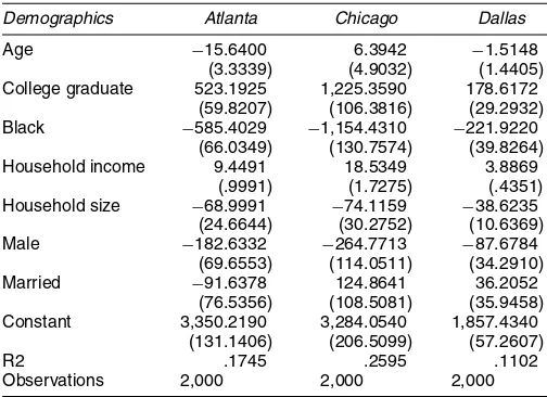
Table 10 reports our structural estimates of the willingness to pay to live in a community whose percentage of adults who are college graduates increases from 10% to 35%. Across all three cities, the college-educated are willing to pay much more to live in the high human capital areas. In Chicago, college graduates are willing to pay $1,225 more per year than non-college graduates to live in such a community. This indicates that among migrants there is a significant degree of sorting. High-skilled individuals are sorting into high-skilled
commu-Table 10. Estimates of the Willingness to Pay to Live in a Highly Educated Community
Demographics Atlanta Chicago Dallas
Age −15.6400 6.3942 −1.5148 (3.3339) (4.9032) (1.4405) College graduate 523.1925 1,225.3590 178.6172
(59.8207) (106.3816) (29.2932) Black −585.4029 −1,154.4310 −221.9220
(66.0349) (130.7574) (39.8264) Household income 9.4491 18.5349 3.8869
(.9991) (1.7275) (.4351) Household size −68.9991 −74.1159 −38.6235
(24.6644) (30.2752) (10.6369) Male −182.6332 −264.7713 −87.6784
(69.6553) (114.0511) (34.2910) Married −91.6378 124.8641 36.2052
(76.5356) (108.5081) (35.9458) Constant 3,350.2190 3,284.0540 1,857.4340
(131.1406) (206.5099) (57.2607) R2 .1745 .2595 .1102 Observations 2,000 2,000 2,000
NOTE: Each column of the table presents a separate ordinary least squares regression. The dependent variable is a migrant’s willingness to pay per year for an increase from 10% to 35% of community members who are college graduates, holding all other housing product attributes constant. Standard errors are reported in parentheses. The omitted category is a white, noncol-lege graduate who is female and not married. Household Income is measured in thousands of 1989 dollars.