SCHEDULING TRAJECTORIES ON A PLANAR SURFACE
WITH MOVING OBSTACLES
by
Emmanuel Stefanakis
Abstract. An algorithm for scheduling the trajectory of a point object, which moves on a plane surface comprising of moving obstacles, is introduced. Different quantitative criteria may be met by the schedule, e.g., the course connecting two individual locations being the shortest in length, the least expensive, the fastest as regard to its duration, etc. A prototype system that implements the algorithm is presented. Several example scenarios are also discussed.
Keywords. Spatio-temporal modeling, graphs, trajectory schedule, optimum paths, moving objects.
1. Introduction
The scheduling of an object (e.g., a vessel) trajectory is a common problem in human navigation and appears very often in applications such as Cartography, Logistics, Robotics and Geographic Information Systems (GIS). Moving between two physical locations can be, basically, accomplished based on various alternative schedules. Each schedule can be characterized and quantitatively described by some objective criteria. For instance, we may look for – to name a few:
9 the shortest, longest, fastest, or least expensive trajectory connecting the two locations,
9 a trajectory that departs from the start location at time ts, and arrives
at destination at time td,
9 a trajectory, which further adds to the previous one the constraint to cross an intermediate location at time ti and reside there for the time interval [ti, tj].
Obviously, there are three additional parameters that should be clarified, before we browse for the trajectory that meets the criteria above. These describe (a) the dimensions of the space where movement takes place, (b) the constraints of movement, and (c) the dynamic nature of space in time.
depending on the application – one, two, two and a half (for curved surfaces, like the earth) or three dimensions in general. In this study, we limit the discussion on movements in a two-dimensional (plane) surface. All concepts can be readily extended and applied to spaces of higher dimensionality (Stefanakis and Kavouras 1995).
As for the constraints of movement, the trajectory connecting two physical locations may be limited to the chains of an existing linear network or not. In the former case, graph theory can be applied to simulate the movement (Johnson 1977, Gibbons 1985, Sedgewick 1990, Rich and Knight 1991, Russell and Norvig 1995). In the latter case, where the movement is not confined to a linear network, existing raster-based (Warntz 1961, Lindgren 1967, Goodchild 1977, Church et al. 1992, van Bemmelen et al. 1993, Douglas 1994ab) or vector-based (Mitchel and Papadimitriou 1991) approaches may be applied. In this study, we examine trajectories in space, and we apply an approach, recently introduced by Stefanakis and Kavouras (1995, 2002). This algorithm is based on the degeneration of the space under study into a network, which can be simulated by a weighted graph, so that algorithms of graph theory and artificial intelligence can be easily adopted to indicate the optimum path(s) for the desired trip.
Finally, as for the dynamic nature of space in time, there are two alternatives. In the first alternative, the space is static, in the sense that the cost of movement per unit of movement (e.g., one meter) remains unchanged over time everywhere in space. In the second alternative, the cost of movement changes over time. The cost of movement is described through a (spatial) cost model (Stefanakis and Kavouras 2002). Obviously, time is a parameter of the cost model. In this study, we examine a simple scenario, where the cost model applies the function of Euclidean distance. That is, the cost of movement (cAB)
from a location A(xA,yA) to a location B(xB,yB) is equal to:
Additionally, we assume that the space comprises a set of moving obstacles, which constraint the access to specific regions (covered by the obstacles) during specific temporal intervals.
constrained by a set of static obstacles, i.e., the islands and continents; and by a set of moving obstacles, i.e., the other vessels.
The discussion is organized as follows. Section 2 describes the algorithm for scheduling the trajectory of an object in a dynamic space with obstacles. Section 3 presents a prototype system which implements the algorithm and several example scenarios generated by the system. Finally, Section 4 concludes the discussion and proposes some hints for future research.
2. The Algorithm
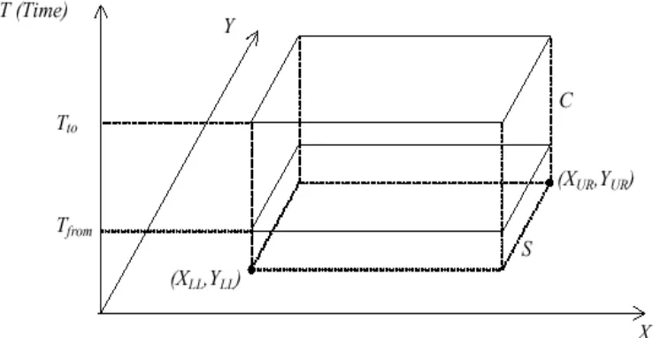
Assume a two-dimensional plane surface S (Figure 1). For simplicity reasons, the surface is orthogonal – with its borders parallel to the X,Y-axes – and described through two pairs of (x,y) coordinates, the lower left (or south west – XLL, YLL) and the upper right (or north east – XUR, YUR) corners. The space is considered during a temporal interval [Tfrom, Tto], defined by a pair of time instances, the Tfrom and Tto, where Tto is subsequent to Tfrom. We call this
period of time as space life. Hence, a spatio-temporal cube C defined by the triples (XLL, YLL, Tfrom) and (XUR, YUR, Tto) is considered.
Figure 1. The space-time.
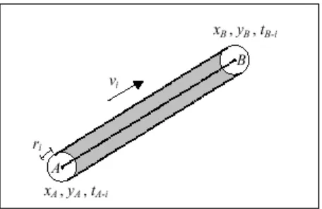
MOi has a circular shape with a radius ri, and carries out a straight route with a constant velocity vi. Specifically, each obstacle MOi is defined by the following set of parameters:
( ri, xfrom-i , yfrom-i , tfrom-i , xto-i , yto-i , tto-i )
where the triples (xfrom-i , yfrom-i , tfrom-i) and (xto-i , yto-i , tto-i) correspond to the starting and ending locations of the obstacle MOi in space-time.
Figure 2 presents an example obstacle MOi with radius ri on surface S (a projective view), which travels from point A(xA,yA) to point B(xB,yB), during the temporal interval [tA-i,tB-i] . The object velocity is constant and equal to:
)
What we are looking for is the schedule (if any) of a point object, which moves on the surface S and its course: (a) connects two specific locations in space, (b) falls inside the spatio-temporal cube C, (c) satisfies the schedule criteria, and (d) does not hit any moving object.
Figure 2. An example of a moving obstacle.
applicable to a dynamic space. As stated previously, the discussion is limited to a plane surface, which comprises a set of moving obstacles of circular shape. The schedule refers to a point object, which moves on this surface and does not hit any moving obstacle at any time. Notice that obstacles size may be enlarged appropriately to include the moving object size – if the latter is not a point object – and/or the security distance (buffer zone) between the point object and the obstacles themselves (to avoid collision).
The algorithm consists of the five steps, which are described in the following Subsections:
1. Establishment of a network in space 2. Formulation of the travel cost model
3. Computation of the temporal intervals during which nodes and edges are not accessible
4. Solving the network
5. Determination of the schedule
2.1 Establishment of a network in space
The inconvenience of movement in space is the infinite number of spots (i.e., point locations or nodes), involved in the determination of a path. The proposed solution (Stefanakis and Kavouras 1995, 2002) to overcome this problem is based on the technique of discretization of space. Discretization (Laurini and Thompson 1992, Worboys 1995) is the process of partitioning the continuous space into a finite number of disjoint areas or volumes (cells), whose union results in the space. By representing each of these cells with one node (e.g., its center point), a finite set of nodes is generated.
Obviously, the number of nodes depends on the size of the cell. If these nodes are interconnected through edges, a linear network is established, and appropriate algorithms available in graph theory and artificial intelligence can be applied to support the navigation. How nodes are interconnected is related to the degrees of freedom characterizing the movement. In this study we adopt a common scheme, which is based on the regular grid tessellation. More details can be found in Stefanakis and Kavouras 2002.
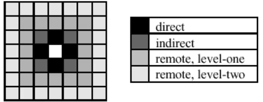
neighbors with common vertices; and (c) remote neighbors. The level of proximity to the cell of reference characterizes remote neighbors.
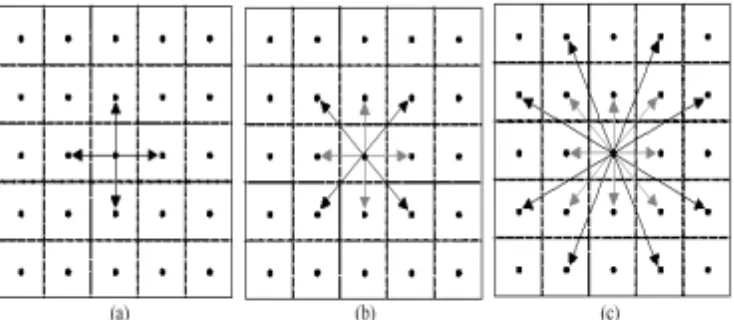
For instance, level-one (level-two) remote neighbors are the cells, which are direct or indirect neighbors of the direct or indirect neighbors of the cell of reference (of the level-one remote neighbors of the cell of reference). Interconnecting the direct neighbors leads to a set of four directions of movement from each node (rook’s move is allowed – Figure 5a). Interconnecting the indirect neighbors adds another set of four directions (queen’s move is allowed – Figure 5b). Interconnecting the level-one remote neighbors adds another set of eight directions of movement (queen’s+knight’s moves are allowed – Figure 5c). An exhaustive network would interconnect all direct, indirect and remote (of any level) neighbors.
Figure 3. Establishing the network nodes. The space (a), the tessellation superimposed on the space (b), and the resulting nodes (c).
Figure 5. Four (a), eight (b) and sixteen (c) directions of movement.
2.2 Formulation of the travel cost model
The travel cost model assigns weights to the edges of the network established in the previous step. Its form depends on both the space under study and the application needs. Some representative examples of travel cost models are:
9 the model of distance (assign the overall distance) 9 the model of time (assign the overall time)
9 the model of expenses (assign the overall expenses) 9 the model of risk (assign a measure for the overall risk)
In each case the space under study consists of areas that are characterized by a weight, which indicates the cost of movement across them per unit of movement; and depends on the travel cost model in use. A detailed analysis is can be found in Stefanakis and Kavouras 2002.
2.3 Computation of the temporal intervals during which nodes and edges are not accessible
After the network has been established, the obstacles are considered in order to compute all those temporal intervals during which nodes and edges are not accessible. This information is needed when the network is solved in Step 4, so that the schedule for the moving object is determined in Step 5.
All nodes and edges locations are compared against all moving obstacles locations in time. At the end of this comparison, each individual node and edge of the network is assigned a list of temporal intervals during which it is not accessible, because an obstacle intersects it.
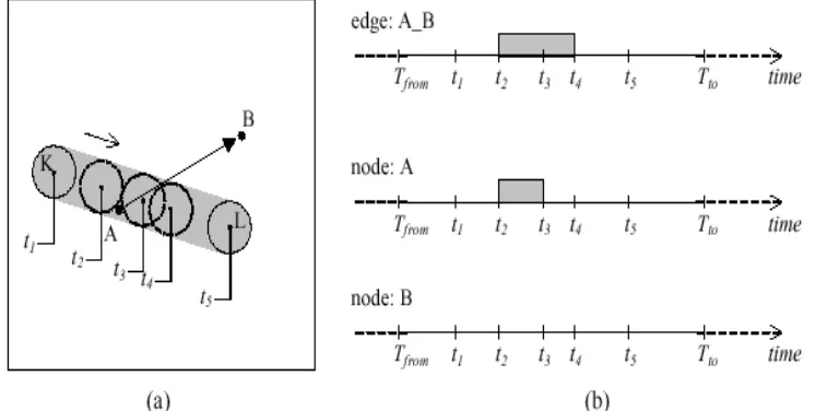
Figure 6 presents an example of two nodes A, B and the edge A_B connecting them. An obstacle moves from point K to point L. As it is shown, the obstacle covers node A during the temporal interval [t2,t3] and intersects the edge A_B during the temporal interval [t2,t4]. During these temporal intervals the corresponding node and edge are not accessible.
Figure 6. An example of a moving object (a), and the temporal intervals during which nodes A,B and edge A_B are not accessible (b).
2.4 Solving the network
not accessible. In this step the actual solving of the network is performed. For this reason, appropriate algorithms available in graph theory and artificial intelligence can be applied. In our study we make use of Ford’s algorithm (Ford and Fulkerson 1962).
Provided a graph G(N, E) (where N, E the sets of nodes and edges constituting the graph respectively), and c(m,n) the cost of traversing the edge m_n, starting from node m and ending to node n, Ford suggests the following algorithm to find the minimum accumulated cost of each network node n (denoted by C[n]) for the trip from a start node no:
The complexity of Ford’s algorithm depends on the number of both the nodes and edges of the network and is equal to O(|N| |E|).
In this study, we extend Ford’s algorithm to solve the spatio-temporal network. By executing the algorithm, each node of the network is assigned a list of temporal intervals, during which the node is accessible from the moving object with the minimum accumulated cost for the trip from the start node no. We call these intervals as accessible temporal intervals. Obviously, the temporal intervals during which nodes and edges are not accessible (computed in the previous step) are taken into account.
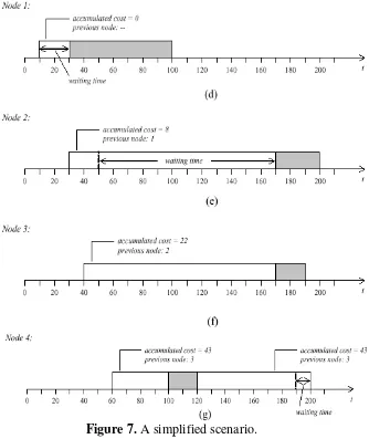
Provided that the trip starts at time 10, the moving object can reside at node 1 during part or the whole interval defined by time 10 and the next time when instance node 1 is not accessible. Therefore, the accessible temporal interval for the moving object at node 1 is [10,30] (Figure 7d,c). The accumulated cost for node 1 is equal to 0 and there is no previous node.
Considering the movement along the edge 1_2, the following apply. The moving object may depart from node 1 at any time during the interval [10,30]. The edge 1_2 is accessible all the time (Figure 7c). Provided that the duration of traversing edge 1_2 is equal to 20, node 2 can be reached at any time during the interval [30,50]. Node 2 is accessible all this period. The accumulated cost at node 2 will be 0+8=8. Additionally, the moving object may reside at node 2 until the next time instance when the node is not accessible. Therefore, the accessible temporal interval for the moving object at node 2 is extended to [30,170] (Figure 7e).
Considering the movement along the edge 2_3, the following apply. The moving object may depart from node 2 at any time during the interval [30,170]. The edge 2_3 is accessible all the time (Figure 7c). Provided that the duration of traversing edge 2_3 is equal to 10, node 3 can be reached at any time during the interval [40,180]. The accumulated cost at node 3 will be 8+14=22. However, node 3 is not accessible during the interval [170,190]. Therefore, the accessible temporal interval for the moving object at node 3 is reduced to [40,170] (Figure 7f).
Considering the movement along the edge 3_4, the following apply. The moving object may depart from node 3 at any time during the interval [40,170]. The edge 3_4 is accessible all the time (Figure 7c). Provided that the duration of traversing the edge 3_4 is equal to 20, node 4 can be reached at any time during the interval [60,190]. The accumulated cost at node 4 will be 22+21=43. However, node 4 is not accessible during the interval [100,120]. Therefore, the object may depart from node 3 during the intervals [40,100-20] (or [40,80]) and [120,170] (in here we assume that departure from a node is not allowed when the edge to traverse and the opposite edge node are not accessible). This results in the accessible temporal interval for the moving object at node 4 being split to [60,100] and [120,190] (Figure 7g). Additionally, the latter is extended to [120,200], based on the previous discussion.
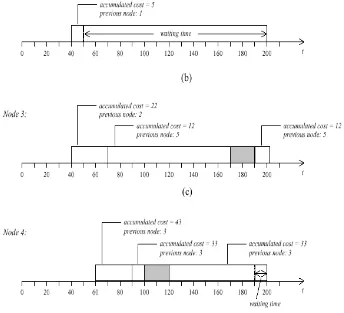
Figure 8b shows the accessible temporal interval for node 5. The moving object may depart from node 1 at any time during the interval [10,30]. However, edge 1_5 is not accessible during the interval [0,20]. Hence, the object must wait at node 1 until t=20. Provided that the duration to traverse the edge is equal to 20, node 5 can be reached at any time during the interval [40,50]. This interval is extended appropriately (to the end of the network life), since node 5 is always accessible.
Node 2 remains unchanged (Figure 7e). Node 3 is now accessible from both nodes 2 and 5. New accessible temporal intervals for the moving object at node 3 are computed by considering the edge 5_3. These are intersected to the ones shown in Figure 7f. The intervals with the minimum accumulated cost dominate. The result of the intersection is shown in Figure 8c. Notice that, in the new network, node 3 can be accessed from node 2 for the temporal interval [40,70], with an accumulated cost of 22; and node 3 for the temporal interval [70,170] and [190,200] with an accumulated cost of 12.
Node 4 is assigned new accessible temporal intervals according to the new state of node 3. As shown in Figure 8d, three accessible temporal intervals are assigned to node 4: [60,90], [90,100] and [120,200], with accumulated costs of 43, 33 and 33, respectively.
2.5 Determination of the schedule
After the network has been solved, the schedule for the moving object can be determined, taking into consideration the criteria of movement. Specifically, the previous step has generated for each network node j (where j=1,2,…,N) a set of n consecutive and disjoint temporal intervals, during which node j is accessible (reachable) by the moving object. Each of these intervals [tji-from, tji-to] (where i=1,2,…,n) has assigned the accumulated cost of movement for the trip from the start node s (cji) and the corresponding previous node (pji), i.e.,
node j: {[tj1-from, tj1-to, cj1, pj1], [tj2-from, tj2-to, cj2, pj2], [tj3-from, tj3-to, cj3, pj3], …, [t jn-from, tjn-to, cjn, pjn]}
This set can be exploited to determine the schedule. The next paragraphs describe some common scenarios.
< tdi-from, cdi, locd >
where locd is the location of the destination node. The process is applied recursively to the node pdi, etc., until start node s is reached. The triplets at T describe the movement of the object. Notice that the cost assigned to the edges of the network may be their length or the expenses to traverse them (e.g., expressed in petrol consumption), etc. In the former case, the shortest in length trip is scheduled. In the latter case, the least expensive trip is scheduled.
In order to schedule the fastest trip, we choose the first temporal interval assigned to the destination node d. Then we add to an empty stack T – describing the trip – the following triplet:
< td1-from, cd1, locd >
The process is applied recursively to the node pd1, etc., until start node s is reached. The triplets at T describe the movement of the object.
In order to schedule the trip that takes the moving object at destination at time ta, we choose the temporal interval k, assigned to the destination node, which contains time ta (i.e., ta 0¸[tdk-from, tdk-to]) Then we add to an empty stack T – describing the trip – the following triplet:
< ta, cdk, locd >
The process is applied recursively to the node pdk, etc., until start node s is reached. The triplets at T describe the movement of the object.
3. Prototype System and Example Scenarios
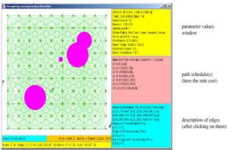
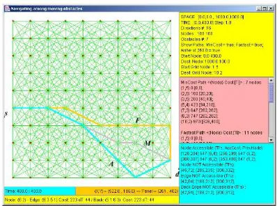
Figure 9. The interface of the system.
Figure 10 shows the values of the parameters that are read by the system for the example in Figure 9. The spatio-temporal cube is defined by the triplet (0,0,0) and (1000,1000,400). Cell size is equal to 100x100 (Figure 3), and 16 directions of movement are considered (Figure 5c). Start and destination points are located at (0,400) and (1000,100) respectively. Their closest network nodes are considered as start and destination nodes (see Figure 10). The start time for the trip is equal to 0. The velocity of the moving object is constant and equal to 5 distance_units/time_units. The system is asked to compute only the minimum cost schedule. Eight moving obstacles are considered. The first of them (id = 1) has a radius of 60 units, and moves from point (0,300) to point (300,300) during the temporal interval [0,60]. The costs assigned to the edges of the network are equal to their length (Euclidean distance).
Figure 11 presents three schedules for the moving object based on different criteria. With the parameter values listed in Figure 10, the system is asked to simulate the courses of the moving object which satisfy:
9 Course F: the fastest cost trip (i.e., the trip that takes the moving object at destination node at the earliest possible).
9 Course A: the arrive at 260 trip (i.e., the trip that takes the moving object at destination node at time 260).
Figure 11. Three schedules for the moving object based on different criteria.
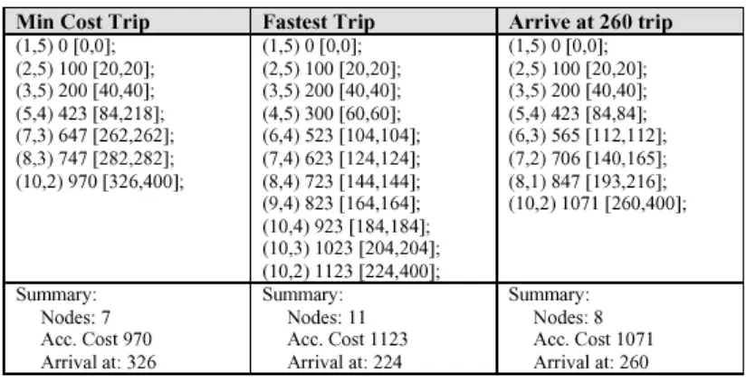
Table 1 presents the courses computed by the system. Each course is described by a set of records:
<(x,y) c [ta, td]>
Table 1. Three courses descriptions for the moving object in Figure 11.
4. Conclusion
This paper introduces an algorithm for scheduling the trajectory of a point object, which moves on a plane surface comprising of moving obstacles. The schedule may be based on various quantitative criteria, e.g., minimum cost course, fastest course, arrive at specific time course, etc. A prototype system that implements the algorithm has been developed and tested through different scenarios.
Future research directions include: (a) the optimal scheduling of trajectories for a set of moving points; (b) the consideration of dynamic travel cost models (Section 2.2), and (c) the optimization of the algorithm.
Acknowledgments.
References:
1. Church, R.L., Loban, S.R., and Lombard, K. (1992) An interface for exploring spatial alternatives for a corridor location problems. Computers and Geosciences, 18, pp. 1095-1105.
2. Douglas, D.H. (1994a) Least-cost path in GIS using an accumulated cost surface and slopelines. Cartographica, 31(3), pp. 37-51.
3. Douglas, D.H. (1994b) The parsimonious path based on the implicit geometry in gridded data and on a proper slope line generated from it, In Proceedings of the 6th International Symposium on Spatial Data Handling, Edinburgh, Scotland, pp. 1133-1140.
4. Ford, L.R., and Fulkerson, D.R. (1962) Flows in Networks (Princeton Univ. Press). 1962.
5. Gibbons, A. (1985) Algorithmic Graph Theory (Cambridge University Press).
6. Goodchild, M.F. (1977) An evaluation of lattice solutions to the problem of corridor location. Environment and Planning A, 9, pp. 727-738.
7. Johnson, D.B. (1977) Efficient algorithms for shortest paths in sparse networks, Journal of the Association of Computing Machinery, 24, pp. 1-13. 8. Laurini, R., and Thompson, D. (1992) Fundamentals of Spatial Information Systems (Academic Press Ltd).
9. Lindgren, E.S. (1967) Proposed solution for the minimum path problem, Harvard Papers in Theoretical Geography, Geography and the Properties of Surfaces Series, 4.
10.Mitchell, J.S.B., and Papadimitriou, C.H. (1991) The weighted region problem: finding shortest paths through a weighted planar subdivision. Journal of the Association for Computing Machinery, 38, pp. 18-73.
11.Rich, E., and Knight, K. (1991) Artificial Intelligence (McGraw-Hill). 12.Russell, S.J., and Norvig, P. (1995) Artificial Intelligence: A Modern Approach (Prentice Hall).
13.Sedgewick, R. (1990) Algorithms (Addison-Wesley).
14.Stefanakis, E., and Kavouras, M. (1995) On the determination of the optimum path in space, In Frank, A., and Kuhn, W., (Ed’s.), Spatial Information Theory: A Theoretical Basis for GIS (COSIT 95) (Springer-Verlag), pp. 241-257.
16.van Bemmelen, J., Quak, W., Van Hekken, M., and van Oosterom, P.
(1993) Vector vs. raster-based algorithms for cross country movement planning. In Proceedings of the AutoCarto 11, Minneapolis, pp. 304-317.
17.Warntz, W. (1961) Transatlantic flights and pressure patterns, The Geographical Review, 51, pp. 187-212.
18.Worboys, M.F. (1995) GIS: A Computing Perspective (Taylor & Francis).
Author: