INFLUENCE OF THE PRECISION OF LIDAR DATA IN SURFACE WATER RUNOFF
ESTIMATION FOR ROAD MAINTENANCE
H. González-Jorge a, *, L. Díaz-Vilariño a, S. Lagüela b, J. Martínez-Sánchez a, P. Arias a
a Applied Geotechnologies Group, Dept. Natural Resources and Environmental Engineering, University of Vigo, Campus Lagoas-Marcosende, CP 36310 Vigo, Spain (higiniog, lucia, joaquin.martinez, parias)@uvigo.es
b Department of Cartographic and Terrain Engineering, University of Salamanca, 05003 Ávila, Spain (sulaguela)@usal.es
Commission III, WG III/2
KEY WORDS: Mobile LiDAR, Point Cloud, runoff, road maintenance.
ABSTRACT:
Roads affect the natural surface and subsurface drainage pattern of a hill or a watershed. Road drainage systems are designed with the objective of reducing the energy generated by the flowing water and the presence of excess water or moisture within the road. A poorly designed drainage may affect to road maintenance causing cut or fill failures, road surface erosion and degrading the engineering properties of the materials with which it was constructed. Surface drainage pattern can be evaluated from Digital Elevation Models typically calculated from point clouds acquired with aerial LiDAR platforms. However, these systems provide low resolution point clouds especially in cases where slopes with steep grades exist. In this work, Mobile LiDAR systems (aerial and terrestrial) are combined for surveying roads and their surroundings in order to provide complete point cloud. As the precision of the point clouds obtained from these mobile systems is influenced by GNSS outages, Gaussian noise with different standard deviation values is introduced in the point cloud in order to determine its influence in the evaluation of water runoff direction. Results depict an increase in the differences of flow direction with the decrease of cell size of the raster dataset and with the increase of Gaussian noise. The last relation fits to a second-order polynomial Differences in flow direction up to 42º are achieved for a cell size of 0.5 m with a standard deviation of 0.15 m.
* Corresponding author.
1. INTRODUCTION
The World Bank (2015) states that road construction includes design, contracting, implementation, supervision, and maintenance. Proper road maintenance contributes to reliable transport at reduced cost. An improperly maintained road can also represent an increased safety hazard to the user, producing more accidents.
The activities of road maintenance can be divided into three main categories: routine works, periodic works, and special works. Routine works are undertaken each year and funded by a recurrent budget. Examples are verge cutting, culvert cleaning, and patching, which is carried out in response to the appearance of cracks of pot-holes. Periodic works include activities undertaken at intervals of several years to preserve the structural integrity of the road such as resealing and overlay works. Special works are the activities for which demand cannot be estimated with in advance, and with reasonable certainty. These activities include emergency works to repair landslides and washouts removal or salting. Too much water flowing in too narrow channels over destabilized soil can produce washouts. Washouts that occur on road surfaces are generally a result of inadequate grading that allows water to channelize rather than staying spread over the whole surface. To avoid this, roads should be properly crowned, road shoulder false berms should be removed or never allowed to form, and cross drainage should be kept free and clear of debris or deposited soil. Roads need to be good quality stable gravel that resists the forces of water and traffic loads.
Drainage installations are sized according to the probability of occurrence of an expected peak discharge during the lifecycle of the installation. This fact is related to the intensity and duration of rainfall events occurring upstream of the road. The water reaching the ground is divided into three paths: some water percolates into the soil, some water evaporates back to the atmosphere, and the rest contributes to the overland flow or runoff. The proportion of rainfall that eventually becomes streamflow is dependent on the size of the drainage area, topography, and soil (Barreiro et al, 2014; Caine 1980).
A popular method to determine flow direction is the D8 algorithm that defines the flow direction in any raster cell through the evaluation of the cell along with its eight neighbouring cells. Digital Elevation Models (DEM) are the input data for the D8 calculation (Douglas 1986; Wang et al, 2014) and water is supposed to follow the steepest descent.
DEM are typically calculated from point clouds that contain geometric information from the environment. Point clouds for these applications are usually provided by means of mobile platforms, aerial and terrestrial. Aerial LiDAR platforms provide results with lower spatial resolution, while terrestrial platforms give higher spatial resolution (Puente et al, 2013; Meesuk et al, 2015). Mobile LiDAR systems combine global navigation satellite systems (GNSS) and inertial measurement units (IMU) for positioning and orientation, with LiDAR systems for range measurements (Petri 2010). All systems are time stamped and boresighted to provide a geo-referenced point cloud.
The quality of the point cloud is affected by external factors that contribute to decrease the precision. One example is the dilution of precision in the GNSS that typically occurs in mountain roads with high slopes, urban areas, and forested roads. The surveying methodology tries to control these aspects, although sometimes it is difficult and the precision of measurements decreases affecting the quality of the point cloud and the derived DEM.
The present work focuses on two aspects. On one hand, it combines the use of airborne LiDAR and terrestrial mobile LiDAR for the evaluation of road runoff. In this way the aerial LiDAR provides information from the top of the mountains surrounding the road and the terrestrial mobile LiDAR provides information from the road slopes and pavement. On the other hand, the influence of LiDAR precision in the evaluation of runoff direction is calculated taking into account the cell size of the DEM and the noise of the LiDAR data. Noise of LiDAR data is artificially introduced according to a Gaussian distribution.
2. AREA OF STUDY
Figure 1 depicts the area of study (42º17’41’’N and 7º35’19’’ W) that corresponds to a mountain road (OU-536) connecting the city of Ourense and the village of A Rúa in Spain. The road presents several slopes, causing major runoff over the road during rainy weather, very common in this region.
Figure 1. Area of study
3. MOBILE LIDAR SYSTEMS
3.1 Aerial LiDAR survey
The National Geographic Institute of Spain (IGN) started a campaign for the acquisition of aerial LiDAR data in 2009, finished in 2012. The sensor used in this area was the LMS-Q680 from Riegl. The scanned field of view is 50º with a scanning frequency of 45 kHz. Point density is 0.5 points per m2, with position precision below 0.2 m. The coordinate system used is UTM – WGS84. Figure 2 shows an example of the aerial point cloud from the area of study.
Figure 2. Aerial point cloud from the area of study.
3.2 Terrestrial LiDAR survey
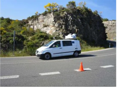
A mobile LiDAR surveying from the area of study was done using and Optech Lynx Mobile Mapper system during 2012. Figure 3 shows the survey van and Figure 4 the resulting point cloud. The Lynx contains an Applanix POS-LV 520 GNSS/IMU for navigation and two Optech LiDAR sensors for range measurement. The main technical specifications are shown in Table 1. It can be observed how GNSS outages decrease precision over 0.1 m.
Figure 3. Survey van with Optech Lynx Mobile Mapper.
Figure 4. Point cloud obtained from the Mobile Terrestrial LiDAR System.
With
GNSS GNSS Outage (1 minute) GNSS X,Y precision (after
post-processing) 0.020 m 0.100 m GNSS Z precision (after
post-processing) 0.050 m 0.070 m IMU Roll and Pitch
precision 0.005 º 0.005 º
IMU Heading precision 0.015 º 0.015 º IMU measurement rate 200 Hz 200 Hz
LiDAR range 200 m 200 m
LiDAR precision 0.008 m 0.008 m Absolute X, Y precision
(GNSS + LiDAR) 0.022 m 0.100 m Absolute Z precision
(GNSS + LiDAR) 0.051 m 0.070 m
LiDAR pulse repetition
rate 500 kHz 500 kHz
LiDAR scan frequency 200 Hz 200 Hz
LiDAR echoes ≤ 4 ≤ 4
Operation temperature -10 ºC to
+ 40 ºC -10 ºC to + 40 ºC
Table 1. Technical specifications of Optech Lynx Mobile Mapper.
The survey was performed at 200 Hz with a pulse repetition rate of 500 kHz for each sensor. The resultant point cloud shows 26,591,026 points with an average point density of 2,084 points/m2. The coordinate system used is UTM – WGS84.
4. DATA PROCESSING
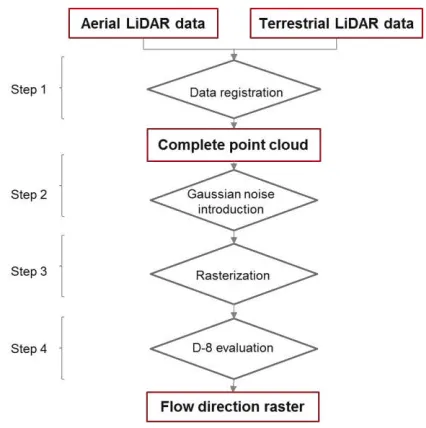
This section deals with the proposed methodology (Figure 5), aiming to evaluate the influence of the precision of point clouds in the estimation of surface drainage pattern in roadsides. The method starts with the registration of aerial and terrestrial point clouds (step 1). Afterwards, Gaussian noise with different standard deviation values is introduced in the point cloud to simulate GNSS outages (step 2). Step 3 consists on generating DEM from point clouds with different cell resolution, which are used as the input to analyse flow directions (Step 4).
Figure 5. Schema of the proposed methodology.
4.1. Aerial and terrestrial data fusion
First step in data processing consists on fusing the terrestrial and aerial mobile LiDAR point clouds. Coarse registration was done by selecting three points from the pavement at the corners of horizontal traffic signs. Fine registration was done using Iterative Closest Point (ICP) algorithm. Cloud Compare software was used for this operation. The final point cloud shows 27,056,827 points (Figure 6).
Figure 6. Terrestrial (blue) and aerial (white) mobile LiDAR point clouds registered in one dataset.
4.2. Generation of Gaussian noise
As the main aim of this work is to evaluate the influence of the precision of point clouds in the estimation of water runoff, point clouds are not submitted to pre-processing operations such as noise removal or filtering.
Gaussian noise is directly introduced in the point cloud in order to simulate the decrease in precision related with GNSS outages. Noise is equally introduced in X, Y and Z coordinates.
Random numbers are generated in MatLAB according different standard deviations and a Gaussian distribution to simulate the noise. The values of the standard deviations taken into account are 0.003 m, 0.005 m, 0.007 m, 0.010 m, 0.020 m, 0.030 m, 0.040 m, 0.050 m, 0.060 m, 0.080 m, 0.100, and 0.150 m. Figure 7 shows a section of the point cloud where points from the original point cloud are represented in white while points from a noised point cloud are showed in black.
Figure 7. Original road – slope profile (white) and noised profile (black)
4.3. Generation of DEM from the point cloud
Third step consists on rasterizing the previous noised point clouds to obtain Digital Elevation Models, which are the input to the evaluation of the influence of LiDAR data precision in surface water runoff estimation.
The rasterization process starts by organizing the point clouds into a uniform XY grid. Next, a nearest neighbour algorithm is used to determine the points belonging to each cell. The algorithm calculates the Euclidean distance between each node of the matrix and the neighbourhood points. The height assigned to each grid cell corresponds to the mean height of the points belonging to each cell. A nearest neighbour Figure 8 shows an example of a raster layer generated from the case study.
Figure 8. DEM with cell resolution of 2 m.
Cell sizes between 0.5 m and 5 m, with an interval of 0.5m, are generated to evaluate the influence of cell resolution. Figure 9 exhibits the relation between the number of cells and the resolution.
Figure 9. Relation between the number of cells of the DEM and cell resolution.
4.4. D8 evaluation
The D8 algorithm is based on the evaluation of the maximum terrain gradient for each cell of a DEM to approximate the primary flow direction (O`Callaghan 1984). It is a grid based algorithm extensively used in Geographic Information Systems (GIS) due to its simplicity and reliability.
For a given grid cell, the D8 algorithm approximates the primary flow direction by choosing the direction to the neighbor with maximal 2D gradient. Figure 10 schematizes the flow calculation with D8 algorithm. For example, the flow direction in the central pixel, with value 19, is down ward. The gradient is maximum towards the pixel directly below with value 17.
Figure 10. Flow directions evaluated with D8 algorithm.
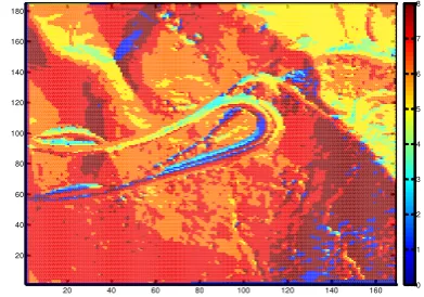
The implementation of the algorithm is performed in MatLAB. Figure 11 shows the results of a runoff evaluation with a cell size of 3 m. Each direction is codified from 1 to 8 counter clockwise beginning at (0, 0).
20 40 60 80 100 120 140 160 20
40 60 80 100 120 140 160 180
0 1 2 3 4 5 6 7 8
Figure 11. Runoff directions from a raster with a grid size of 3 m from an original point cloud.
4.5. Differences in runoff evaluation with D8
Final step of the methodology consists on evaluating the differences of flow directions between raster datasets from the original point cloud and those with Gaussian noise. The comparison is carried out for each cell size considered in this study and differences range between 0º to 180º.
Figure 12 shows de differences in the evaluation of runoff direction between the original data and a simulated point cloud with Gaussian noise with standard deviation of 0.1 m.
20 40 60 80 100 120 140 160
Figure 12. Differences in D8 evaluation.
5. RESULTS AND DISCUSSION
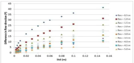
The difference in flow direction versus the size of the DEM cell for different standard deviations is shown in Figure 13. According to the results, differences in flow direction decrease with the increase of cell size. In addition, differences in flow direction increase with the increasing of standard deviation. For a resolution of 0.5 m, flow differences range between approximately 5º for standard deviations of 0.003 m to 42º for 0.150 m. A noisy point cloud clearly contributes negatively to the precision of flow direction.
Figure 13. Difference in flow direction versus DEM resolution.
Figure 14 exhibits the relation in flow direction versus the standard deviation of the noise. Results are fitted to second-order polynomial (Table 2), making necessary to parametrize the behaviour and determine the precision of D8 evaluation depending on the cell size and precision of surveyed data.
Figure 14. Difference in flow direction versus standard deviation of Gaussian noise.
Table 2. Fitting parameters to equation of the form:
difference = a·std2 + b·std + c
CONCLUSIONS
In this work, the influence of the precision of LiDAR data is evaluated and parameterized for runoff estimation. The analysis is carried out for a real case study where terrestrial and aerial LiDAR data is combined in order to complete the available data.
The surface drainage pattern of the road and its surroundings is determined by using the D8 algorithm under different conditions of LiDAR precision. Gaussian noise is artificially generated in the original point cloud to determine its influence in the evaluation of D8 algorithm. Standard deviation of the noise ranges between 0.003 m and 0.15 m. Furthermore, different cell sizes are taken into account, from 0.5 m to 5 m, in order to evaluate the influence of raster resolution in runoff estimation.
The differences in runoff evaluation are analysed for each cell size and averaged to obtain a single value. Differences between the D8 results from the original point cloud and those point clouds with added Gaussian noise increase with the decrease of cell size and the increase of standard deviation. Differences range between 5º to 42º for standard deviations of 0.003 m and 0.150 m. Cell resolution in this case is 0.5 m. On the other hand, differences in flow direction change between 42º and 10º for 0.15 m standard deviation and cell size between 0.5 m and 5 m, respectively.
ACKNOWLEDGEMENTS
Authors want to give thanks to the Xunta de Galicia (CN2012/269; R2014/032) and Spanish Government (Grant No: TIN2013-46801-C4-4-R; ENE2013-48015-C3-1-R; FPU: AP2010-2969).
REFERENCES
Barreiro, A., Domínguez, J. M., Crespo, A. J. C., González-Jorge, H., Roca, D., Gómez-Gesteira, M. 2014. Integration of UAV photogrammetry and SPH modelling of fluids to study runoff on real terrains. PlosONE, 9(11), e 111031.
Caine, N. 1980. The rainfall intensity. Geografiska Annaler.
Series A, Physical, 62(1/2), 23 – 24.
Douglas, D. H. 1986. Experiments to locate ridges, channels to create a new type of digital elevation model. Cartographica,
23(4), 29 – 61.
Meesuk, V., Vojinivic, Z., Mynett, A. E., Abdullah, A. F. 2015. Urban flood modeling combining top-view LiDAR data with ground-view SfM. Advances in Water Resources, 75, 105 –
117.
O’Callaghan, J. F. and Mark, D. M. 1984. The extraction of drainage networks from digital elevation data. Computer Vision
Graphics and Image Processing, 28(3), 323 – 344.
Petri, G. 2010. Mobile mapping systems: An introduction to the technology. Geoinformatics Magazine, 13(1), 32 – 43.
Puente, I., González-Jorge, H., Martínez-Sánchez, J., Arias, P. 2013. Review of mobile mapping and surveying technologies.
Measurement, 46(7), 2127 – 2145.
Wang, J., González-Jorge, H., Lindenbergh, R., Arias-Sánchez, P., Menenti, M. 2014. Geometric road runoff estimation from laser mobile mapping data. ISPRS Annals of the Photogrammetry, Remote Sensing, and Spatial Information
Sciences, II-5, 385 – 391.
World Bank (2015);
http://www.worldbank.org/transport/roads/con&main.htm#road maint