Amitrajeet A. Batabyal *
Department of Economics,Utah State Uni6ersity,3530Old Main Hill,Logan,UT84322-3530,USA
Received 3 November 1997; received in revised form 12 November 1998; accepted 23 November 1998
Abstract
We now know that from a functional standpoint, jointly determined ecological – economic systems (ecosystems) cycle over time. However, because this recognition has been recent, the ecological economics literature contains very few formal studies of the management of cyclical ecosystems. Consequently, the objective of this paper is to use renewal theory to examine two ways of analyzing the optimal management of cyclical ecosystems. © 1999 Elsevier Science B.V. All rights reserved.
Keywords:Cyclical ecological – economic system; Optimal management; Renewal theory JEL classification:Q30; D80
1. Introduction
Recent research in ecology has led to major
revisions in the theory of ecosystem1 succession
proposed by Clements (1916). The Clementsian view of succession envisaged an orderly process in which species assemblages progressively moved towards a climax. The assemblage and the
charac-teristics of the climax species are determined by climate and soil conditions. In the Clementsian view of succession, the two primary ecosystem functions are exploitation and conser6ation. The
exploitation function emphasizes the rapid colo-nization of recently disturbed areas, and the
con-servation function refers to the gradual
accumulation of energy and materials.
However, as Holling (1986, 1995) and Holling et al. (1995) have noted, recent research in ecology has stressed the need for two additional functions.
One function is that of creati6e destruction or
release. This concerns the release of accumulated
* Tel.: +1-435-797-2314; fax:+1-435-797-2701. E-mail address:[email protected] (A.A. Batabyal)
1In the rest of this paper, I shall use the terms ‘ecosystem’
and ‘ecological-economic system’ interchangeably.
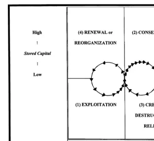
Fig. 1. The ecosystem cycle. Source: Holling (1986, p. 307 and 1995, p. 22).
biomass and nutrients by agents such as forest fires, insect pests, and severe pulses of grazing.
The other function is that of reorganization or
renewal. This relates to the reorganization of nu-trients so that these nunu-trients are available in the next phase of exploitation. As a result of the addition of these two functions, from a functional standpoint, the ecosystem succession picture can now be described by a four box cycle (see Fig. 1). It is important to note that during this cycle, biological time flows very unevenly. An ecosystem moves slowly from exploitation (box 1) to conser-vation (box 2), then very quickly to release (box 3), once again quickly to renewal (box 4), and finally back to exploitation (box 1). In the process of moving from box 1 to box 2, the ecosystem becomes progressively more organized. Second, as the system moves from box 1 to box 4, the stored capital of biomass and nutrients in the ecosystem rises.
Given the existence of this cycle, if ecosystem management is to be effective, then it must incor-porate this essential cyclicity in the design of management policies. In addition to this, there are two other features of ecosystems that managers need to account for in the design and the conduct of policies. The first feature is that ecological –
economic systems are jointly determined. As
co-tem management. In particular, it tells us that management actions and policies need to be
adaptable to changing circumstances. This
need for adaptability is very important because, as Holling (1995) has noted, rigid management policies may be successful in the short run, but they inexorably lead to less resilient ecosys-tems and more dependent societies in the long run.
Despite the significance of managing jointly determined, cyclical ecosystems from an adap-tive standpoint, there are very few formal stud-ies of the management of such systems. In particular, there do not appear to be many studies that have analyzed the ways in which the management function is affected by the pres-ence of uncertainty. For instance, consider the work of Dixon (1997) on watershed manage-ment, the work of Dixon and Lal (1997) on the management of coastal wetlands, and the work of Nelson (1997) on the management of dry-lands. While these papers are competent sum-maries of the empirical aspects of ecosystem management, they have very little to say about the formal aspects of the management of jointly determined, cyclical ecosystems.
Recently, Brown and Roughgarden (1995),
Perrings and Walker (1995), and Batabyal
(1998) have analyzed formal models of ecosys-tem management. While Brown and Roughgar-den (1995) do provide an ecological – economic analysis of the problem of optimally harvesting a marine resource, their analysis is conducted in
resources. Batabyal (1998) has used his stochas-tic characterization of resilience to show how an ecosystem manager can control the parameters of the management problem to optimally man-age the flow of services provided by an
ecosys-tem. These two papers do use an
ecological – economic approach to the manage-ment problem; moreover, both papers explicitly analyze the role of uncertainty in the ecosystem management problem. Nevertheless, neither pa-per analyzes the essential cyclicity of ecosystems. Given this state of affairs, there is a clear need for studying the management of cyclical
ecosystems. In this paper, I use renewal theory3
to construct and analyze two models of the op-timal management of cyclical ecosystems. Fol-lowing Holling et al. (1995, p. 62), the first model’s cycle may be interpreted as a renewal cycle.4 In contrast to this, the second model
an-alyzes a cycle of economic use.
2. The optimal management of cyclical ecosystems
2.1. The ecosystem cycle
Consider a stylized ecosystem which consists of a number of species. As discussed in Section 1, this ecosystem cycles between the exploitation, conservation, renewal, and reorganization func-tions. As well, this ecosystem provides a flow of services to society over time. The economic
uti-3For more on renewal theory, see Wolff (1989, pp. 52 – 147)
and particularly Ross (1996, pp. 98 – 162).
4Note that ‘renewal cycle’ and ‘ecosystem cycle’ are
differ-ent names for the same phenomenon.
2The term ‘surprise’ is from Holling (1986). For a more
lization of these services results in shocks5 to the
ecosystem. I suppose that these shocks occur in accordance with a renewal process whose
interar-rival time is b. The economic utilization of the
flow of ecosystem services results in benefits and costs to society. The social benefits include those that arise from activities such as boating, fishing, and grazing. The social costs arise from the fact that some of these shocks may result in surprises, and from the increased vulnerability of the ecosys-tem species to future shocks resulting from eco-nomic activities.6
I suppose that whenever the
number of shocks reaches S, the ecosystem
cy-cle — shown in Fig. 1 — closes.7
In other words, shocks can play the role of the creative destruc-tion funcdestruc-tion in the ecosystem cycle. Further, I suppose that when our ecosystem has been
sub-jected to s shocks, an ecosystem manager — or
alternately, a benevolent social planner entrusted with the prudent use of the ecosystem — incurs variable costs8 at the rate of s·c dollars per unit
time. In addition to these variable costs, our
manager incurs a fixed cost ofFdollars when the
cycle closes. The reader should think of F as the
cost of renewal. Thus, from a management per-spective, the social cost of economic activities is the sum of these fixed and variable costs. Our task now is to compute the long-run average social
cost (hereafter ASC) of economic activities that
are incurred by the ecosystem manager.
Recall that a cycle is completed whenever the number of shocks reachesS. As such, the descrip-tion of events contained in the previous para-graph constitutes a renewal – reward process. The
ASC can now be computed by applying the
re-newal – reward theorem to our problem.9 The
re-newal – reward theorem tells us that the expected
long runASCis simply the expected cost incurred
in a cycle divided by the expected time of that cycle. Put differently, we have
ASC= E[cycle cost]
E[cycle length]. (1)
Let Xsdenote the time between the sth and the
(s+1) shock in a cycle. Then the numerator on
the right-hand side of Eq. (1) is given by
E[cycle cost]
=F+E[1cX1+2cX2+3cX3+…+(S-1)cXS−1].
(2)
The right-hand side of Eq. (2) can be simplified to
E[cycle cost]=F+cb(S-1)S
2 . (3)
In order to compute the denominator on the right-hand side of Eq. (1), it suffices to note that the expected length of a cycle is simply the
ex-pected time it takes for S shocks to hit our
ecosystem. Because the mean interarrival time for the shock renewal process is b, we get
E[cycle length]=bS. (4)
Now combining our results from Eq. (3) and
Eq. (4), we get an expression for the ASC. This
expression is
ASC= F
bS+
c(S−1)
2 . (5)
There are two things to note about Eq. (5).
First, as we would expect, ASCequals the sum of
the average fixed and the average variable social costs. Second, if the closure of the ecosystem cycle does not result in any fixed costs, then the mean interarrival time between shocks (b) has no effect
on the ASC.
The ecosystem manager’s goal is to put in place those controls that will, inter alia, improve the
5Some of these shocks may result in surprises. In other
words, these shocks may result in effects that are different from those that were expected by an ecosystem manager. For more on this, see Holling (1986).
6Put differently, the social costs arise from the potential
reduction in the resilience of the ecosystem.
7One can also think of the closure of the cycle in terms of
the strength of these shocks. In this way of looking at the problem, we would say that the cycle closes when the strength of the shocks reachesS.
8Here, and elsewhere in the paper, costs refer to net costs,
i.e., the difference between the gross social costs that economic activities impose on the ecosystem and the gross benefits that such activities bring to society.
9The renewal reward theorem is discussed in Ross (1996,
problem can now be stated. This manager solves
Assuming that a regular minimum exists, the vector of optimal controls (u*1,…,u*n) satisfies
S(u*1,…,u*n)=
'
2F
bc. (7)
The second order conditions to problem (6) are
2F
The first order necessary condition (Eq. (7))
tells us that the manager will choose the n
con-trols so that the number of shocks required to close the ecosystem cycle equals the square root of twice the cost of renewal divided by the product of the mean interarrival time and the marginal cost of the shocks. Eq. (7) also tells us that if the
cost of renewal (F) increases, then the manager
will choose then controls so that the number of
shocks required to close the ecosystem cycle is now higher than before. Finally, the first order condition tells us that if either the mean interar-rival time of the shocks (b) or the marginal cost
of the shocks (c) increases, then the manager’s
optimal response will be to choose the n controls
so that the number of shocks required to close the cycle decreases.
of attempting to influence the number of shocks that are required to close the ecosystem cycle, the manager now follows a different strategy. In par-ticular, this manager attempts to determine the
optimal length of the cycle of use that
accompa-nies the pursuit of economic activities. Put differ-ently, the manager uses time-based policies to
minimize the ASC of economic activities.
Exam-ples of such policies include the regulation of fishing season length, moratoriums on grazing, the fallowing of agricultural land, and the tempo-ral management of forest fires. Note that in con-trast with the cycle of Section 2.1, we are now analyzing an economic use cycle. Our task now is
to compute the long-run ASCthat is incurred by
the ecosystem manager when this manager’s focus is on time rather than on shocks per se.
Once again, I appeal to the renewal – reward theorem. A use cycle is completed upon
regula-tion, i.e. every T time periods. In order to
com-pute E[cycle cost], I first condition on N(T), the total number of shocks that hit our ecosystem by time T. This yields
E[cycle cost /N(T)]=F+cTN(T)
2 , (9)
and hence, the ASCis given by
ASC=F
T+
cT
2b. (10)
Eq. (10) tells us that when the object of study is an economic use cycle, the mean interarrival time (b) affects theASC, irrespective of whether soci-ety does or does not incur fixed costs from the closure of the use cycle.
To determine the optimal length of a use cycle, for example, the optimal length of a fishing
sea-son, the ecosystem manager will choose T to
10Other kinds of management controls will be discussed in
Section 2.2.
11It is possible that the manager may incur certain costs in
minimize the ASC in Eq. (10). In other words,
Once again assuming a regular minimum, the first order necessary condition to problem (10) is
T*=
'
2bFc , (12)
and the second order condition is
2F
T3\0. (13)
Eq. (12) tells us that the optimal length of an economic use cycle equals the square root of twice the product of the mean interarrival time and the fixed cost of closing the cycle divided by the marginal cost of the shocks. This equation also reveals the opposite effect that the marginal cost of shocks (c) and the fixed cost of closing the use cycle (F) have on this optimal cycle length. As the marginal cost of shocks rises, T* falls. To inter-pret this result, consider the case of a fishery. The result says that as fishing becomes more costly to
society — possibly because the intensity with
which it is being pursued rises — a fishery manager responds optimally by reducing the length of the fishing season. In contrast, a rise in the fixed cost of closing the use cycle has the effect of increasing the length of the use cycle. One kind of fixed cost that is associated with the closure of a use cycle is the cost of enforcement. In a fishery this might be the cost borne by a manager to ensure that no boats are fishing after the expiry of the fishing season. The above result says that if this cost rises, then ceteris paribus, the manager will in-crease the length of the use cycle. Finally, an increase in the mean interarrival time of shocks (b) lengthens the use cycle.
3. Discussion
In this paper, I considered two ways of analyz-ing the management of cyclical ecological –
eco-nomic systems. The model of Section 2.1
examined the management function in the context
of Holling’s (Holling, 1986, 1995) four-box ecosystem cycle. The model of Section 2.2 looked at management in the context of an economic use cycle. These models are abstractions; conse-quently they do not tell us everything about the complex world of ecosystem management. The study of ecosystem management is complicated by a number of factors, and it is not possible to analyze all these factors in one or two models. As such, I now briefly discuss four factors that are relevant to the study of ecosystem management.
First, it is important to note that even when a researcher thinks that he or she has identified and specified a management problem correctly, this may not be the case. Second, all theoretical in-quiries necessarily have practical boundaries and this fact ought to be recognized. For instance, the optimal cycle length that is identified in Eq. (12) may not in fact be optimal because the model does not account for shortsightedness and human
greed in the context of ecosystem management.12
Third, as indicated earlier, Holling (1986) has observed that surprise is an essential aspect of ecosystems. Fourth, Holling (1995) has also ob-served that the short-run success in managing an ecosystem can lead to the long-run collapse of the same ecosystem. These two observations should alert us to the fact that the efficacy of managerial actions is circumscribed by our limited ability to predict the future behavior of ecosystems, and our inadequate understanding of the functioning of ecosystems. As Ludwig et al. (1993), Holling (1995), and others have noted, this means that we should be cautious in our approach to ecosystem management, and we should implement manage-ment policies that are adaptable.
4. Conclusions
This paper addressed some aspects of the opti-mal management of cyclical ecosystems from a hitherto unstudied renewal theoretic perspective. In particular, the renewal – reward theorem was
Section 2.1 looked at managerial policies that might be called ‘shock based’. In Section 2.2, the focus was on ‘time-based’ policies. The economics literature on domestic environmental regulation in the presence of uncertainty has demonstrated the
superiority of mixed control instruments in some
situations. This means that a control that is part-price and part-quantity is sometimes superior to a
pure price or a pure quantity control.13 Is this
insight relevant in the context of ecosystem man-agement? This is a question on which additional research is needed. This research will shed light on the desirability of adopting policies that are, for instance, ‘shock based’ and ‘time based’.
Interconnected ecosystems are poorly under-stood by practicing ecosystem managers. Inter alia, this is because ecosystem managers have to guess the values of the parameters of theoretical models. I have not discussed the problem of esti-mating the parameters of this paper’s models so that the resulting models are useful in terms of their predictive power. Clark (1990, p. 340) has noted the importance of this ‘identification’ prob-lem in the context of fisheries. However, this identification problem is more general and it ap-plies to all ecosystems. Consequently, coordinated
interdisciplinary research by ecologists and
economists is needed to make theoretical models more useful from a practical standpoint.
Studies of ecosystem management which incor-porate these aspects of the problem into the anal-ysis will permit richer analyses of the management of cyclical ecosystems. In turn, such studies will
Research Grant program at Utah State Univer-sity, and the Utah Agricultural Experiment
Sta-tion, Utah State University, Logan, UT
84322-4810, by way of grant UTA 024. Approved
as journal paper c 6002. The usual disclaimer
applies.
References
Batabyal, A.A., 1995. Leading issues in domestic environmen-tal regulation: a review essay. Ecol. Economics 12, 23 – 39. Batabyal, A.A., 1998. On species substitutability, resilience, and the optimal management of ecological – economic sys-tems. Mathematical Computer Modelling (in press). Batabyal, A.A., Beladi, H., 1998. The optimal management of
a class of aquatic ecological – economic systems. Depart-ment of Economics, Utah State University. Mimeo. Batabyal, A.A., Yoo, S.J., 1994. Renewal theory and natural
resource regulatory policy under uncertainty. Economics Lett. 46, 237 – 241.
Batabyal, A.A., Yoo, S.J., 1996. Renewal theory and natural resource regulatory policy under uncertainty: a corrigen-dum. Economics Lett. 52, 119.
Brown, G., Roughgarden, J., 1995. An ecological economy: notes on harvest and growth. In: Perrings, C., Ma¨ler, K., Folke, C., Holling, C.S., Jansson, B. (Eds.), Biodiversity Loss. Cambridge University Press, Cambridge, UK. Clark, C.W., 1990. Mathematical Bioeconomics, 2nd ed.,
Wi-ley, New York, USA.
Clements, F.E., 1916. Plant succession: an analysis of the development of vegetation. Carnegie Institute of Washing-ton Publication 242, 1 – 512.
Dasgupta, P., 1996. The economics of the environment. Envi-ron. Dev. Economics 1, 387 – 428.
Dixon, J., 1997. Analysis and management of watersheds. In: Dasgupta, P., Ma¨ler, K. (Eds.), The Environment and Emerging Development Issues, vol. 2. Oxford University Press, Oxford, UK.
Dixon, J., Lal, P., 1997. The management of coastal wetlands: economic analysis of combined ecologic – economic sys-tems. In: Dasgupta, P., Ma¨ler, K. (Eds.), The Environment and Emerging Development Issues, vol. 2. Oxford Univer-sity Press, Oxford, UK.
13A tax is an example of a price control and a quota is an
Holling, C.S., 1986. The resilience of terrestrial eco-systems: local surprise and global change. In: Clark, W.C., Munn, R.E. (Eds.), Sustainable Development of the Biosphere. Cambridge University Press, Cambridge, UK.
Holling, C.S., 1995. What barriers? What bridges? In: Gunder-son, L.H., Holling, C.S., Light, S.S. (Eds.), Barriers and Bridges to the Renewal of Ecosystems and Institutions. Columbia University Press, New York, USA.
Holling, C.S., Schindler, D.W., Walker, B., Roughgarden, J., 1995. Biodiversity in the functioning of ecosystems: an ecological synthesis. In: Perrings, C., Ma¨ler, K., Folke, C., Holling, C.S., Jansson, B. (Eds.), Biodiversity Loss. Cam-bridge University Press, CamCam-bridge, UK.
Ludwig, D., Hilborn, R., Walters, C., 1993. Uncertainty, resource exploitation, and conservation: lessons from his-tory. Science 260, 17 – 36.
Nelson, R., 1997. The management of drylands. In: Dasgupta, P., Ma¨ler, K. (Eds.), The Environment and Emerging Development Issues, vol. 2. Oxford University Press, Ox-ford, UK.
Perrings, C., 1996. Ecological resilience in the sustainability of economic development. In: Faucheux, S., Pearce, D., Proops, J. (Eds.), Models of Sustainable Development. Edward Elgar, Cheltenham, UK.
Perrings, C., Walker, B., 1995. Biodiversity loss and the eco-nomics of discontinuous change in semiarid rangelands. In: Perrings, C., Ma¨ler, K., Folke, C., Holling, C.S., Jansson, B. (Eds.), Biodiversity Loss. Cambridge University Press, Cambridge, UK.
Ross, S.M., 1996. Stochastic Processes, 2nd ed., Wiley, New York, USA.
Wolff, R.W., 1989. Stochastic Modeling and the Theory of Queues. Prentice-Hall, Englewood Cliffs, USA.
.