Full Terms & Conditions of access and use can be found at
http://www.tandfonline.com/action/journalInformation?journalCode=ubes20
Download by: [Universitas Maritim Raja Ali Haji], [UNIVERSITAS MARITIM RAJA ALI HAJI
TANJUNGPINANG, KEPULAUAN RIAU] Date: 11 January 2016, At: 20:58
Journal of Business & Economic Statistics
ISSN: 0735-0015 (Print) 1537-2707 (Online) Journal homepage: http://www.tandfonline.com/loi/ubes20
Multiple Imputation of Missing or Faulty Values
Under Linear Constraints
Hang J. Kim, Jerome P. Reiter, Quanli Wang, Lawrence H. Cox & Alan F. Karr
To cite this article: Hang J. Kim, Jerome P. Reiter, Quanli Wang, Lawrence H. Cox & Alan F. Karr (2014) Multiple Imputation of Missing or Faulty Values Under Linear Constraints, Journal of Business & Economic Statistics, 32:3, 375-386, DOI: 10.1080/07350015.2014.885435
To link to this article: http://dx.doi.org/10.1080/07350015.2014.885435
View supplementary material
Accepted author version posted online: 20 Feb 2014.
Submit your article to this journal
Article views: 188
View related articles
View Crossmark data
Multiple Imputation of Missing or Faulty Values
Under Linear Constraints
Hang J. K
IMDuke University and National Institute of Statistical Sciences, Durham, NC 27708 ([email protected])
Jerome P. R
EITERand Quanli W
ANGDepartment of Statistical Science, Duke University, Durham, NC 27708 ([email protected]; quanli@stat. duke.edu)
Lawrence H. C
OXand Alan F. K
ARRNational Institute of Statistical Sciences, Research Triangle Park, NC 27709 ([email protected]; [email protected])
Many statistical agencies, survey organizations, and research centers collect data that suffer from item nonresponse and erroneous or inconsistent values. These data may be required to satisfy linear constraints, for example, bounds on individual variables and inequalities for ratios or sums of variables. Often these constraints are designed to identify faulty values, which then are blanked and imputed. The data also may exhibit complex distributional features, including nonlinear relationships and highly nonnormal distribu-tions. We present a fully Bayesian, joint model for modeling or imputing data with missing/blanked values under linear constraints that (i) automatically incorporates the constraints in inferences and imputations, and (ii) uses a flexible Dirichlet process mixture of multivariate normal distributions to reflect complex distributional features. Our strategy for estimation is to augment the observed data with draws from a hypothetical population in which the constraints are not present, thereby taking advantage of computation-ally expedient methods for fitting mixture models. Missing/blanked items are sampled from their posterior distribution using the Hit-and-Run sampler, which guarantees that all imputations satisfy the constraints. We illustrate the approach using manufacturing data from Colombia, examining the potential to preserve joint distributions and a regression from the plant productivity literature. Supplementary materials for this article are available online.
KEY WORDS: Edit; Hit-and-Run; Mixture; Survey; Truncation.
1. INTRODUCTION
Most economic datasets suffer from missing data. For ex-ample, among the plants surveyed in the 2007 U.S. Census of Manufactures and across all six-digit NAICS industries, 27% of plants are missing total value of shipments, 32% of plants are missing book values of assets, and 42% of plants are missing cost of materials. As is well known (Little and Rubin 2002), using only the complete cases (all variables are observed) or available cases (all variables for the par-ticular analysis are observed) can cause problems for statis-tical inferences, even when variables are missing at random (Rubin1976). By discarding cases with partially observed data, both approaches sacrifice information that could be used to in-crease precision. Further, using only available cases complicates model comparisons, since different models could be estimated on different sets of cases; standard model comparison strate-gies do not account for such disparities. For data collected with complex survey designs, using only available cases complicates survey-weighted inference, since the original weights generally are no longer meaningful for the available sample.
An alternative to complete/available cases is to fill in the miss-ing items with multiple imputations (Rubin 1987). The basic idea is to simulate values for the missing items by sampling re-peatedly from predictive distributions. This createsm >1 com-pleted datasets that can be analyzed or, as relevant for many data producers, disseminated to the public. When the
impu-tation models meet certain conditions (Rubin 1987, chap. 4), analysts of themcompleted datasets can make valid inferences using complete-data statistical methods and software. Specif-ically, the analyst computes point and variance estimates of interest with each dataset and combines these estimates using simple formulas developed by Rubin (1987). These formulas serve to propagate the uncertainty introduced by missing data and imputation through the analyst’s inferences. See Reiter and Raghunathan (2007) for a review of multiple imputation.
In many settings, imputations of numerical variables must respect linear constraints. These constraints arise particularly in the context of editing faulty data, that is, values that are not plau-sible (e.g., a plant with one million employees, or a large plant with an average salary per employee of $1 million) or that are inconsistent with other values on the data file (e.g., an establish-ment reporting an entry year of 2012 that also reports nonzero employment in earlier years). For example, the U.S. Census Bu-reau requires numerical variables to satisfy an extensive set of ratio constraints intended to catch errors in survey reporting or data capture in the Census of Manufactures, the Annual Survey
© 2014American Statistical Association Journal of Business & Economic Statistics
July 2014, Vol. 32, No. 3 DOI:10.1080/07350015.2014.885435
Color versions of one or more of the figures in the article can be found online atwww.tandfonline.com/r/jbes.
375
of Manufactures, and the Services Sectors Censuses (SSC) in the Economic Census (Winkler and Draper1996; Draper and Winkler 1997; Thompson et al.2001). Examples of non-U.S. economic data products, subject to editing, include the Survey of Average Weekly Earnings of the Australian Bureau of Statistics (Lawrence and McDavitt1994), the Structural Business Survey of Statistics Netherlands (Scholtus and Goksen2012), and the Monthly Inquiry Into the Distribution and Services Sector of the U. K. Office for National Statistics (Hedlin2003).
Despite the prevalence and prominence of such contexts, there has been little work on imputation of numerical variables under constraints (De Waal, Pannekoek, and Scholtus2011). Most sta-tistical agencies use hot deck imputation: for each record with missing values, find a record with complete data that is similar on all observed values, and use that record’s values as impu-tations. However, many hot deck approaches do not guarantee that all constraints are satisfied and, as with hot deck impu-tation in general, can fail to describe multivariate relationships and typically result in underestimation of uncertainty (Little and Rubin2002). Tempelman (2007) proposed to impute via trun-cated multivariate normal distributions that assign zero support to multivariate regions not satisfying the constraints. This ap-proach presumes relationships in the data are well-described by a single multivariate normal distribution, which for skewed eco-nomic variables is not likely in practice even after transforma-tions (which themselves can be tricky to implement because the constraints may be difficult to express on the transformed scale). Raghunathan et al. (2001) and Tempelman (2007) proposed to use sequential regression imputation, also called multiple impu-tation by chained equations (Van Buuren and Oudshoorn1999), with truncated conditional models. The basic idea is to impute each variableyj with missing data from its regression on some
function of all other variables{ys :s=j}, enforcing zero
sup-port for the interval values ofyj not satisfying the constraints.
While more flexible than multivariate normal imputation, this technique faces several challenges in practice. Relations among the variables may be interactive and nonlinear, and iden-tifying these complexities in each conditional model can be a laborious task with no guarantee of success. Furthermore, the set of specified conditional distributions may not correspond to a coherent joint distribution and thus is subject to odd theoret-ical behaviors. For example, the order in which variables are placed in the sequence could impact the imputations (Baccini et al.2010).
In this article, we propose a fully Bayesian, flexible joint modeling approach for multiple imputation of missing or faulty data subject to linear constraints. To do so, we use a Dirichlet process mixture of multivariate normal distributions as the base imputation engine, allowing the data to inform the appropri-ate number of mixture components. The mixture model allows for flexible joint modeling, as it can reflect complex distribu-tional and dependence structures automatically (MacEachern and M¨uller1998), and it is readily fit with MCMC techniques (Ishwaran and James2001). We restrict the support of the mix-ture model only to regions that satisfy the constraints. To sample from this restricted mixture model, we use the Hit-and-Run sam-pler (Boneh and Golan1979; Smith1980), thereby guarantee-ing that the imputations satisfy all constraints. We illustrate the constrained imputation procedure with data from the Colombian
Annual Manufacturing Survey, estimating descriptive statistics and coefficients from a regression used in the literature on plant productivity.
The remainder of the article is organized as follows. In Section 2, we review automatic editing and imputation processes, which serves as a motivating setting for our work. In Section3, we present the constrained Dirichlet process mixture of multivari-ate normals (CDPMMN) multiple imputation engine, including the MCMC algorithm for generating imputations. In Section 4, we apply the CDPMMN to the Colombian manufacturing data. In Section 5, we conclude with a brief discussion of future research directions.
2. BACKGROUND ON DATA EDITING
Although the CDPMMN model is of interest as a general es-timation and imputation model, it is especially relevant for na-tional statistical agencies and survey organizations—henceforth all called agencies—seeking to disseminate high-quality data to the public. These agencies typically dedicate significant re-sources to imputing missing data and correcting faulty data be-fore dissemination. For example, Granquist and Kovar (1997) estimated that national statistical agencies spend 40% of the total budget for business surveys (20% for household surveys) on edit and imputation processes, and in an internal study of 62 products at Statistics Sweden, Norberg (2009) reported that the agency allocated 32.6% of total costs in business surveys to editing processes. Improving these processes serves as a pri-mary motivation for the CDPMMN imputation engine, as we now describe.
Since the 1960s, national statistical agencies have leveraged the expertise of subject-matter analysts with automated methods for editing and imputing numerical data. The subject-matter experts create certain consistent rules, called edit rules or edits, that describe feasible regions of data values. The automated methods identify and replace values that fail the edit rules.
For numerical data, typical edit rules includerange restric-tions, for example, marginal lower and upper bounds on a single variable,ratio edits, for example, lower and upper bounds on a ratio of two variables, andbalance edits, for example, two or more items adding to a total item. In this article, we consider range restrictions and ratio edits, but not balance edits. Formally, letxij be the value of thejth variable for theith subject, where
i=1, . . . , n, and j =1, . . . , p. For variables with range re-strictions, we haveLj ≤xij ≤Uj, whereUjandLjare
agency-fixed upper and lower limits, respectively. For any two variables (xij, xik) subject to ratio edits, we have Lj k ≤xij/xik≤Uj k,
where againUj kandLj kare agency-fixed upper and lower
lim-its, respectively. An exemplary system of ratio edits is displayed inTable 1. These rules, defined by the U.S. Census Bureau for data collected in the SSC, were used to test editing routines in 1997 Economic Census (Thompson et al.2001).
The set of edit rules defines a feasible region (convex poly-tope) comprising all potential records passing the edits. A po-tential data recordxi =(xi1, . . . , xip)′satisfies the edits if and
only if the constraintsAxi≤bfor some matrixAand vectorb
are satisfied. Any record that fails the edits is replaced (imputed) by a record that passes the edits.
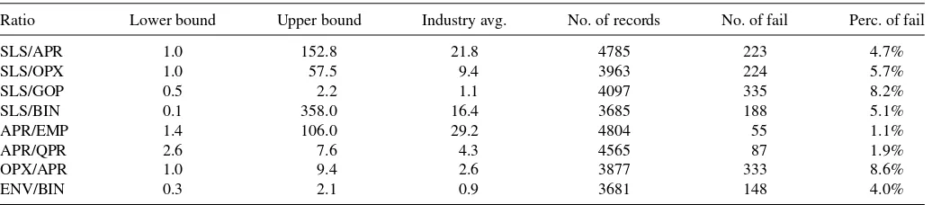
Table 1. Exemplary ratio edits in the SSC
Ratio Lower bound Upper bound Industry avg. No. of records No. of fail Perc. of fail
SLS/APR 1.0 152.8 21.8 4785 223 4.7%
SLS/OPX 1.0 57.5 9.4 3963 224 5.7%
SLS/GOP 0.5 2.2 1.1 4097 335 8.2%
SLS/BIN 0.1 358.0 16.4 3685 188 5.1%
APR/EMP 1.4 106.0 29.2 4804 55 1.1%
APR/QPR 2.6 7.6 4.3 4565 87 1.9%
OPX/APR 1.0 9.4 2.6 3877 333 8.6%
ENV/BIN 0.3 2.1 0.9 3681 148 4.0%
NOTE: SLS=sales/receipts, APR=annual payroll, OPX=annual operating expenses, GOP=purchases, EMP=employment, QPR=first quarter payroll, BIN=beginning inventory, and ENV=ending inventory.
Finding records that fail rules is straightforward, at least conceptually, with automated routines and modern computing. However, identifying the faulty values within any record (the error localization procedure) and correcting those erroneous values (the imputation procedure) are far more complicated tasks. Among national statistical agencies, the most commonly used error localization procedure is that of Fellegi and Holt (1976), who developed a set covering algorithm that identifies the minimum number of values to change in the data to sat-isfy all edit rules. Fellegi and Holt (1976) error localization algorithms are the basis for many automated edit systems, in-cluding the U.S. Census Bureau’s SPEER (Draper and Winkler 1997), Statistics Canada’s GEIS (Whitridge and Kovar1990), Spanish National Statistical Institute’s DIA (Garcia-Rubio and Villan1990), Statistics Netherlands’ CherryPi (De Waal2000), and Istituto Nazionaledi Statistica’s SCIA (Manzari2004). We do not discuss error localization steps further, as our concern is with the imputation procedure; that is, we assume that the erroneous fields of survey data that violate edit rules have been detected and blanked by the agency, and we focus on imputing the blanked values.
3. MODEL AND ESTIMATION
We now present the CDPMMN imputation engine. We begin in Section3.1by reviewing Dirichlet mixtures of multivariate normal distributions without any truncation or missing data. We adopt the model in Section3.2to handle truncation and present an MCMC algorithm to estimate the model, again assuming no missing data. We modify this algorithm in Section3.3.to ac-count for missing data, making use of a Hit-and-Run algorithm in the MCMC steps. We discuss several implementation issues in Section3.4.
3.1 Dirichlet Process Mixtures of Normals Without Truncation
LetYn= {y1, . . . ,yn}comprisencomplete observations not
subject to edit constraints, where each yi is a p-dimensional
vector. To facilitate modeling, we assume that the analyst stan-dardizes each variable before modeling to have observed mean equal to 0 and observed standard deviation equal to 1; see Ap-pendix B in the supplementary material for details of the stan-dardization. We suppose that each individualibelongs to exactly one ofK <∞latent mixture components. Fori=1, . . . , n, let
zi ∈ {1, . . . , K}indicate the component of individuali, and let
πk=Pr(zi =k). We assume thatπ=(π1, . . . , πK) is the same
for all individuals. Within any component k, we suppose that thepvariables follow a component-specific multivariate normal distribution with meanµkand variancek. Let=(μ, ,π),
whereμ=(µ1, . . . ,µK) and=(1, . . . , K).
Mathemati-cally, the finite mixture model can be expressed as
yi |zi, μ, ∼N(yi |µzi, zi) (1) zi |π ∼Multinomial(π1, . . . , πK). (2)
Marginalizing overzi, this model is equivalent to
p(yi |) = K
k=1
πkN(yi |µk, k). (3)
As a mixture of multivariate normal distributions, the model is flexible enough to capture distributional features like skewness and nonlinear relationships that a single multivariate normal distribution would fail to encode.
To complete the Bayesian specification, we require prior dis-tributions for. As suggested by Lavine and West (1992), for (µk, k) we use
µk |k ∼N(µ0, h−1k) (4)
k ∼Inverse Wishart(f, ), (5)
wheref is the degrees of freedom,=diag(φ1, . . . , φp), and
φj ∼ Gamma(aφ, bφ) (6)
with meanaφ/bφ forj =1, . . . , p. These conditionally
conju-gate prior distributions simplify the MCMC computations. We defer discussion of these hyperparameter values until Section 3.2, when we present the constrained model.
For the component weights,π, we use the stick-breaking rep-resentation of a truncated Dirichlet process (Sethuraman1994; Ishwaran and James2001), shown in (7)–(8).
πk =vk
g<k
(1−vg) fork=1, . . . , K (7)
vk ∼Beta(1, α) fork=1, . . . , K−1; vK =1 (8)
α∼Gamma(aα, bα). (9)
Here, (aα, bα) are analyst-supplied constants. Following Dunson
and Xing (2009), we recommend setting (aα =0.25, bα=
0.25), which represents a small prior sample size and, hence, vague specification for Gamma distributions. This ensures that
the information from the data dominates the posterior distribu-tion (Escobar and West 1995). The specification of prior dis-tributions in (7)–(9) encourages πk to decrease stochastically
withk. Whenαis very small, most of the probability inπ is allocated to the first few components, thus reducing the risks of over-fitting the data as well as increasing computational effi-ciency. We note that Dirichlet process distributions are widely used for mixture models in economic analyses (e.g., Hirano 2002; Gilbride and Lenk2010).
As a prior distribution for π=(π1, . . . , πK), one
also could use a symmetric Dirichlet distribution, π ∼
Dir(a/K, . . . , a/K), for example, witha=1. We expect that imputations based on the truncated Dirichlet process prior distri-bution and this symmetric Dirichlet distridistri-bution generally will not differ noticeably. We use the truncated Dirichlet process prior distribution primarily because (i) it has worked well in other applications of mixture models for multiple imputation of missing data (Si and Reiter2013; Manrique-Vallier and Reiter forthcoming) and (ii) in our experience, it facilitates reasonably fast MCMC convergence.
With specified hyperparameters, the model can be estimated using a Gibbs sampler, as each full conditional distribution is in closed form; see Ishwaran and James (2001).
3.2 Dirichlet Process Mixtures of Normals With Truncation
The model in Section3.1has unrestricted support and, hence, is inappropriate for imputation under linear constraints. Instead, when yiis restricted to lie in some feasible regionA, we need
to replace (3) with
where I(·)=1 when the condition inside the parentheses is true, andI(·)=0 otherwise. Here,h(A, ) is the normalizing
Equivalently, using the representation conditional onzi, we need
to replace (1) with
We leave all other features of the model as described in (2) and (4)–(9).
Unfortunately, due to the truncation, full conditional dis-tributions depending on the likelihood do not have conjugate forms, thus complicating the MCMC. To avoid computation withh(A, ), we use a data augmentation technique developed
by O’Malley and Zaslavsky (2008) in which we (i) conceive of the observed values as a sample from a larger, hypothetical sample not subject to the constraints, (ii) construct the hypo-thetical sample by augmenting the observed data with values from outside ofA, and (iii) use the augmented data to estimate parameters using the usual, unconstrained Gibbs sampler. With appropriate prior distributions, the resulting parameter estimates correspond to those from the CDPMMN model.
Specifically, we assume that there exists a hypothetical sam-ple of unknown sizeN > nrecords,YN = {Yn, YN−n}, where
number of cases inAhas distribution
n|N, ,A ∼ Binomial(N, h(A, )). (15)
We use the prior distribution suggested by Meng and Zaslavsky (2002) and O’Malley and Zaslavsky (2008),p(N)∝1/N for
N > n, so that
N−n|n, ,A ∼ Negative Binomial (n,1−h(A, )).
(16)
With this construction, we can estimatewithout computing
h(A, ) using an MCMC algorithm. LetZN = {Zn, ZN−n}be
the set of membership indicators corresponding toYN, where
Zn= {z1, . . . , zn}andZN−n= {zn+1, . . . , zN}. For each group
the MCMC algorithm proceeds with the following Gibbs steps.
S1. Fork=1, . . . , K, sample values of (µk, k) from the full
S4. Givenπ, sampleαfrom the full conditional,
distribution following the approach suggested by O’Malley and Zaslavsky (2008). Specifically, based on the result in (16), we draw each (zi,yi)∈(ZN−n, YN−n) from a negative
binomial data-generating process. To begin, setcin=cout =
0. Then, perform the following steps.
S6.1. Drawz∗ ∼Multinomial(π
For the prior distributions in (4)–(6), we recommend using a prior mean ofµ0=0 since each variable is mean-centered, usingf =p+1 degrees of freedom to ensure a proper distri-bution without overly constraining, and settingh=1 mostly for convenience. We recommend setting (aφ, bφ) to be
mod-est but not too small, so as to allow substantial prior mass at modest-sized variances. Following Dellaportas and Papageor-giou (2006), we useaφ =bφ=0.25. In the Colombia data
il-lustration, results were insensitive to other sensible choices of hyperparameter values; details of the sensitivity analysis are in Appendix A, available as online supplementary material.
3.3 Accounting for Missing Data: Hit-and-Run Algorithm
Having developed an MCMC algorithm for fitting the CDP-MMN model without any missing values, we now extend to include imputation of missing data or, equivalently, imputation of blanked values due to edit rules. Here, we assume the miss-ing data mechanism is ignorable (Rubin1976). Without loss of generality, suppose that the firsts≤nrecords inYnhave some
missing values. LetYs = {y1, . . . ,ys}be these firstsrecords,
andYn−s = {ys+1, . . . ,yn}be the set of fully observed records.
For eachyi ∈Ys, let yi =(yi,0,yi,1), whereyi,0comprises the
missing values and yi,1comprises the observed values. Finally,
letYs,0= {y1,0, . . . ,ys,0}, and letYs,1= {y1,1, . . . ,ys,1}.
Formally, we seek to estimate the posterior distribution,
f(Ys,0, YN−n, ZN, , , α, N |Ys,1, Yn−s,A). We do so in two
steps, namely (i) given a draw ofYs,0satisfyingA, draw values
of (YN−n, ZN, , , α, N) using S1 – S6 from Section3.2, and
(ii) given a draw of (YN−n, ZN, , , α, N), draw imputations
forYs,0satisfyingAusing a Metropolis version of the
Hit-and-Run (H&R) sampler (Chen and Schmeiser1993). Thus, we only need to add an imputation step to the MCMC algorithm from Section3.2, as we now describe.
We begin by finding the region of feasible imputations for each yi,0, which we write asAi = {yi,0;yi =(yi,0,yi,1)∈A}.
For systems of linear constraints like those inTable 1and typ-ically employed in edit-imputation contexts,Ai can be defined using matrix algebra operations; see Appendix C, supplemen-tary material, for an illustrative example. For more complex linear constraints, feasible regions can be found by linear pro-graming and related optimization techniques.
The H&R sampler proceeds as follows. At any iterationtof the MCMC sampler, we presume the current values of each yi,0,
say y(i,t0), wherei=1, . . . , s, satisfy the constraints; see Section 3.4for a suggestion to initialize the chain at feasible values. The basic idea of the H&R sampler is to pick a random direction inRpi, wherep
i is the number of variables in yi,0; follow that
direction starting from y(i,t0) until hitting the boundary of Ai, say at some pointb(i,t0); and, sample a new point along the line
segment with end points (y(i,t0),b (t)
i,0). For convexAi, the selected
point is guaranteed to be inside the feasible region. Formally, we implement this process via the Metropolis step in S7 below.
S7. For i=1, . . . , s, update each current value y(i,t0) with a Metropolis accept/reject step as follows.
S7.1. Propose a directiond∗∼r(·) wherer(·) is a uniform distribution on the surface of the unit sphere inRp.
S7.2. Find the set of candidate proposal distances, which we write as(d∗,y(i,t0))= {λ∈R: y a uniform distribution with the density 1/M
{(d∗,y(i,t)0)}, whereMis a Lebesgue measure. S7.4. Accept or reject the proposal yqi,0= y
(t)
i,0+λ∗d ∗with
the acceptance probabilityρi, where
ρi =min
Note that the acceptance probability can be calcu-lated by using the fact that the conditional distri-bution of yi,0 is proportional to that of yi, that is,
p(yi,0|zi, μ, ,Ai)∝p(yi |zi, μ, ,A) as in (12).
After canceling common terms, the acceptance prob-ability simplifies to ρi=min{1,N(y
Because the H&R sampler randomly moves in any direction, it can cover multivariate spaces more efficiently than typical Gibbs samplers that move one direction in each conditional step. The efficiency gain can be substantial when the sample space is a convex polytope and when variables are highly correlated or sharply constrained (Chen and Schmeiser1993; Berger1993). Lov´asz and Vempala (2006) proved that the H&R sampler mixes fast, and that mixing time does not depend on the choice of starting points. Hence, for imputing multivariate data subject to the constraints, the H&R sampler offers a potentially significant computational advantage over typical Gibbs steps.
To obtainmcompleted datasets for use in multiple imputa-tion, one selectsmof the sampledYs,0after MCMC convergence.
These datasets should be spaced sufficiently to be approximately independent (given the observed data). This involves thinning
the MCMC samples so that the autocorrelations among param-eters are close to zero.
3.4 Implementation Issues
In this section, we discuss several features of implementing the CDPMMN imputation engine, beginning with the choice of
K. SettingK too small can result in insufficient flexibility to capture complex features of the distributions, but settingKtoo large is computationally inefficient. We recommend initially setting K to a reasonably large value, say K=50. Analysts can examine the posterior distribution of the number of unique values of zi across MCMC iterates to diagnose if K is large
enough. Significant posterior mass at a number of classes equal toKsuggests that the truncation limit should be increased. We note that one has to assume a finiteKbecause of the truncation; otherwise, the model can generate arbitrary components with nearly all mass outsideA.
One also has to select hyperparameter values, as we discussed in Section3.2. Of note here is the value ofhin (4), which deter-mines the spread of mean vectors. For example, small values of
hgenerally imply that, a priori,µkcan be far fromµ0.
Empiri-cally, our experience is that small values ofhcan generate large values ofN, the number of augmented values, which can slow the MCMC algorithm. We recommend avoiding very smallh, say by settingh >0.1, to reduce this computational burden. As noted in Section 3.2and the sensitivity analysis in Appendix A, our application results are robust to changes ofhand other hyperparameters.
To initialize the MCMC chains when using the H&R sampler, we need to choose a set of points all within the polytope defined byA. To do so, we find the extreme points of the polytope along each dimension by solving linear programs (Tervonen et al. 2013), and set the starting point of the H&R chain as the arith-metic mean of the extreme points. We run this procedure for find-ing startfind-ing values usfind-ing the R package “hitandrun” (available at
http://cran.r-project.org/web/packages/hitandrun/index.html).
In our empirical application, other options of finding starting points within the feasible region, including randomly weighted extreme points or vertex representation, do not change the final results.
With MCMC algorithms it is essential to examine conver-gence diagnostics. Due to the complexity of the models and many parameters, as well as the truncation and missing val-ues, monitoring convergence of chains is not straightforward. We suggest that MCMC diagnostics focus on the draws ofN,
α, the ordered samples ofπ, and, when feasible, values of the
π-weighted averages of µk and k, for example, kπkµk,
rather than specific component parameters, {µk, k}. Specific
component parameters are subject to label switching among the mixture components, which complicates interpretation of the components and MCMC diagnostics; we note that label switch-ing does not affect the multiple imputations.
4. EMPIRICAL EXAMPLE: COLOMBIAN MANUFACTURING DATA
We illustrate the CDPMMN with multiple imputation and analysis of plant-level data from the Colombian Annual
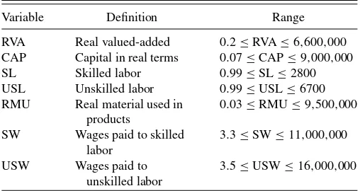
Manu-Table 2. Variables in the Colombian Annual Manufacturing Survey, with range restrictions that we introduce for illustration
Variable Definition Range
facturing Survey from 1977 to 1991 (except for 1981, for which we have no data). Similar data have been used in analyses of plant-level productivity (e.g., Fernandes2007; Petrin and White 2011). Following Petrin and White (2011), we use the seven variables inTable 2. We remove a small number of plants with missing item data or nonpositive values, so as to make a clean file on which to evaluate the imputations. The resulting annual sample sizes range from 5770 to 6873.
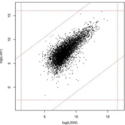
To illustrate the performance of the CDPMMN imputation engine, we introduce range restrictions on each variable (see Table 2) and ratio edits on each pair of variables (seeTable 3) like those used by government agencies in economic data. Limits are wide enough that all existing records satisfy the constraints, thus offering a set of true values to use as a gold standard. However, the limits are close enough to several observed val-ues that the constraints matter, in the sense that estimation and imputation under models that ignore the truncation would have nonnegligible support in the infeasible region.Figure 1displays a typical example of the linear constraints for two variables, log(USW) and log(CAP).
We then randomly introduce missing values in the observed data, and use the CDPMMN imputation engine to implement multiple imputation of missing values subject to linear con-straints. We do so in two empirical studies: a set of analy-ses designed to compare one-off inferences from the imputed and original data (before introduction of missing values), and a repeated sampling experiment designed to illustrate efficiency gains in using the CDPMMN over complete-case methods.
In both studies, we make inferences for unknown pa-rameters according to the multiple imputation inferences of Rubin (1987), which we review briefly here. Suppose that the analyst seeks to estimate some quantity Q, such as a regres-sion coefficient or population mean. Let{D(1), . . . , D(m)}be mcompleted datasets drawn from the CDPMMN imputation engine. Given completed data, the analyst estimates Q with some point estimatorq and estimates its variance withu. For
l=1, . . . , m, letq(l)andu(l)be, respectively, the value ofqand
ucomputed withD(l). The analyst uses ¯qm= m1 ml=1q(
l)to
es-timateQandTm=u¯m+(1+1/m)bmto estimate its variance,
where ¯um=ml=1u(l)/mandbm=ml=1(q(l)−q¯m)2/(m−1).
For large samples, inferences for Qare obtained from the t -distribution, ( ¯qm−Q)∼tνm(0, Tm), where the degrees of
free-dom isνm=(m−1) [1+u¯m/{(1+1/m)bm}]2. Tests of
sig-nificance for multicomponent null hypotheses are derived by
Table 3. Introduced ratio edits in Colombian Manufacturing Survey
Ratio Minimum Maximum Ratio Minimum Maximum
RVA/CAP 7.0e-05 6100 SL/USL 3.0e-03 270
RVA/SL 7.2e-02 500,000 SL/RMU 8.0e-06 1350
RVA/USL 4.2e-02 1,000,000 SL/SW 4.0e-05 1.2
RVA/RMU 6.0e-05 1,300,000 SL/USW 4.0e-06 5.0
RVA/SW 5.9e-05 1000 USL/RMU 1.0e-06 13000
RVA/USW 5.3e-05 3333 USL/SW 1.0e-06 2.5
CAP/SL 2.4e-02 100,000 USL/USW 1.0e-06 1.5
CAP/USL 1.5e-02 333,333 RMU/SW 2.2e-07 1250
CAP/RMU 4.0e-05 1,111,111 RMU/USW 7.1e-08 2500
CAP/SW 1.5e-05 1250 SW/USW 4.0e-03 850
CAP/USW 1.7e-05 250
Li, Raghunathan, and Rubin (1991), Meng and Rubin (1992), and Reiter (2007).
4.1 Comparisons of CDPMMN-Imputed and Original Data
For each yeart =1977, . . . ,1991 other than 1981, letDorig,t
be the original data before introduction of missing values. For each year, we generate a set of missing valuesYs,t by randomly
blanking data fromDorig,tas follows: 1500 records have one
ran-domly selected missing item, 1000 records have two ranran-domly selected missing items, and 500 records have three randomly selected missing items. One can interpret these as missing data or as blanked fields after an error localization procedure. Miss-ingness rates per variable range from 10.2% to 11.5%. This represents a missing completely at random mechanism (Rubin 1976), so that complete-case analyses based only on records with no missing data, that is,Yn−s,t, would be unbiased but
in-Figure 1. The linear constraints for two variables, log(USW) and log(CAP), for 1982 data.
efficient, sacrificing roughly half of the observations in any one year. We note that these rates of missing data are larger than typical fractions of records that fail edit rules, so as to offer a strong but still realistic challenge to the CDPMMN imputation engine.
We implement the CDPMMN imputation engine using the model and prior distributions described in Section3 to create
m=10 completed datasets, each satisfying all constraints. To facilitate model estimation, we work with the standardized nat-ural logarithms of all variables (take logs first, then standardize using observed data).
After imputing on the transformed scale, we transform back to the original scale before making inferences. Of course, we also transform the limits of the linear inequalities to be consistent with the use of standardized logarithms; see Appendix B, avail-able as online supplementary material. We run the MCMC al-gorithm of Section3for 10,000 iterations after a burn-in period, and store every 1000th iterate to obtain them=10 completed datasets. We useK=40 components, which we judged to be sufficient based on the posterior distributions of the numbers of uniquezi among thencases.
We begin by focusing on results from the 1991 survey; re-sults from other survey years are similar.Figure 2summarizes the marginal distributions of log(CAP) in the original and com-pleted datasets. For the full distribution based on all 6607 cases, the distributions are nearly indistinguishable, implying that the CDPMMN completed data approximate the marginal distribu-tions of the original data well. The distribution of the 714 values of log(CAP) inDorigbefore blanking is also similar to those in the three completed datasets.
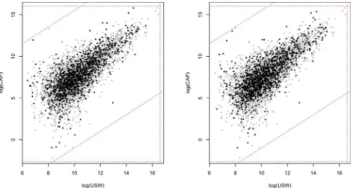
Figure 3 displays a scatterplot of log(USW) versus log (CAP)—at least one of these variables is missing for 20.3% of cases—forDorig and one of the completed datasets; results
for otherD(l)are similar. The overall bivariate patterns are very
similar, suggesting once again the high quality of the imputa-tions. We note that the shape of the joint density implies that a model based on a single multivariate normal distribution, even absent truncation, would not be appropriate for these data.
Figure 4displays scatterplots of pairwise correlations across all variables in the original and three completed datasets. For the full distribution based on all 6607 cases, the correlations are very similar. Correlations based on only the 3000 cases with at least one missing item also are reasonably close to those based on the original data.
Figure 2. Left panel: Distributions of log(CAP) from original data and three completed datasets for all 6607 records in the 1991 data. Right panel: Distributions of log(CAP) for 714 blanked values in the original data and the imputed values in three completed datasets. Boxes include 25th, 50th, and 75th percentiles. Dotted lines stretch from minimum value to 5th percentile, and from 95th percentile to maximum value. The marginal distributions in the imputed datasets are similar to those in the original data.
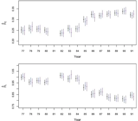
We next examine inferences for coefficients in the regression used by Petrin and White (2011) to analyze plant productivity, namely
log(RVAi)=β0+βClog(CAPi)+βLlog(LABi)+εi,
εi∼N(0, σ2), (17)
where LABi=SLi+USLi. We estimate regressions
indepen-dently in each year. Figure 5 displays OLS 95% confidence intervals fromDorig,tand from the CDPMMN multiply imputed
datasets in each year. For comparison, it also displays intervals based on only the complete cases. The intervals forβbased on the CDPMMN completed datasets are similar to those based on
Dorig, with somewhat wider lengths due to the missing values. For comparison, the complete-case results typically have even wider standard errors.
4.2 Repeated Simulation
The results inFigure 5suggest that the CDPMMN multiple imputation offers more efficient inferences than the complete cases analysis. To verify this further, we perform a repeated sampling study. We assume that the 6607 plants in the 1991 data comprise a population. We then randomly sample 500
indepen-dent realizations ofDorigfrom this population, each comprising
1000 records. For each sampledDorig, we introduce missing
val-ues by blanking one value for 200 randomly selected records, two values for 200 randomly sampled records, and three values for 100 randomly sampled records. We create m=10 com-pleted datasets using the CDPMMN imputation engine using the same approach as in Section4.1, and estimate the regression coefficients in (17) using the multiple imputation point estima-tor. We also compute the point estimates based onDorigand only
the complete cases.
To evaluate the point estimators, for each method we com-pute three quantities for each coefficient inβ=(β0, βC, βL)=
(β0, β1, β2). The first quantity is the simulated bias, Biasj =
500
r=1βˆr,j/500−βpop,j,j =0,1,2, where ˆβr,j is a
method-specific point estimate ofβj in replicationr andβpop,j is the
value of βj based on all 6607 cases. The second quantity is
the total squared error, TSEj =500r=1( ˆβr,j−βpop,j)2. The third
quantity is the total squared distance between the point estimates based on the imputed (or only complete) data and the original data, TSDj =500r=1( ˆβr,j−βˆr,j(orig))2.
Table 4displays the results of the simulation study. All meth-ods are approximately unbiased, with the complete-cases anal-ysis being far less efficient than the CDPMMN multiple im-putation analysis. The CDPMMN multiple imim-putation closely follows the analysis based on the original data.
Figure 3. Plots of log(USW) versus log(CAP) for 1991 data. The left plot displays the original data and the right plot displays one completed dataset. The gray blobs represent records whose values are the same in both plots. The crosses represent the records subject to blanking. The dotted lines show the range restrictions and ratio edits. The distributions are similar.
Figure 4. Plots of correlations among all seven variables for 1991 data. The horizontal coordinates are the correlations in the original data, and the vertical coordinates are the correlations in three completed datasets. Circles represent values forD(1), crosses represent values forD(2),
and triangles represent values forD(3). The left plot uses all 6607 cases and the right plot uses only the 3000 cases with at least one missing item.
Figure 5. Ninety-five percent confidence intervals forβC andβLfrom original data (first displayed interval), CDPMMN multiply imputed data (second displayed interval), and the complete cases (third displayed interval). Using CDPMMN results in similar intervals as the original data, and shorter intervals than the complete cases.
Since the repeated simulation results are based on a missing completely at random (MCAR) mechanism, we also perform a repeated simulation study with a missing at random (MAR) mechanism; see Appendix D in the supplementary materials for details. The performance of the CDPMMN imputations are akin to those inTable 4: point estimates are approximately unbiased with roughly a 30% increase in variance due to missing data. The complete-cases analysis results in biased estimates.
For both the MCAR and MAR scenarios, we also examine results for multiple imputation by chained equations using the
MICE software (Van Buuren and Groothuis-Oudshoorn2011) in R. We use the default implementation, which is based on predictive mean matching using linear models. In any com-pleted dataset, there are usually a handful of imputed values that result in violations of the inequality constraints. Agencies seeking to release data clean of violations would have to change these values manually, whereas the CDPMMN imputation au-tomatically respects such constraints. Nonetheless, we found that point estimators from the predictive mean matching MICE and the CDPMMN imputation performed quite similarly on our
Table 4. Properties of point estimators across the 500 simulations for the original data, the CDPMMN multiple imputation, and the complete cases analysis
β0 βC βL
Bias TSE TSD Bias TSE TSD Bias TSE TSD
Original data −0.007 4.03 − 0.001 0.21 − −0.001 0.60 −
CDPMMN −0.002 5.19 1.31 −0.001 0.27 0.07 0.001 0.78 0.20 Complete-cases −0.006 8.55 4.71 0.000 0.48 0.26 0.002 1.38 0.75
three evaluation measures, both in the MCAR and MAR scenar-ios. Of course, the performance of any method depends on the features of the data. Determining general conditions when the CDPMMN outperforms MICE, and vice versa (after manually fixing violations), is a topic worthy of further study.
5. CONCLUDING REMARKS
The empirical analyses of the Colombia manufacturing data suggest that the CDPMMN offers a flexible engine for generat-ing coherent imputations guaranteed to respect linear inequal-ities. We expect the CDPMMN to be computationally feasible with efficient parallel computing when the number of variables is modest, say on the order of 40 to 50. For larger numbers of variables, analysts may need to use techniques other than the CDPMMN, for example, models based on conditional indepen-dence assumptions such as Bayesian factor models (Aguilar and West2000). We note that the general strategy of data augmen-tation combined with a Hit-and-Run sampler can be applied to any Bayesian multivariate model. In contrast, we do not view the number of records as a practically limiting factor, because the computations can be easily parallelized or implemented with GPU computing (Suchard et al. 2010). If computation-ally necessary, and potenticomputation-ally for improved accuracy, analysts can split the data into subsets of rows, for example, by indus-try classifications, and estimate the model independently across subsets.
As with any imputation-model specification, it is prudent to examine the fit of the CDPMMN model for the particular con-text. As described in Gelman et al. (2005), one can compare the marginal distributions of the observed and imputed values as a “sanity check.” Highly dissimilar distributions can suggest the model does not describe the data well. One also can com-pute posterior predictive checks (e.g., He et al.2010; Burgette and Reiter2010; Si and Reiter2013). As described by Si and Reiter (2013), the basic idea is to use the imputation model to generate not only Ys but an entirely new full dataset, that is,
create a completed datasetD(l) =(Ys(l), Yn−s) and a replicated
datasetR(l) in which bothYs andYn−s are simulated from the
imputation model. After generating many pairs (D(l), R(l)), one compares eachR(l)with its correspondingD(l)on statistics of interest, such as regression coefficients and tail area probabili-ties. When the statistics are dissimilar, the diagnostic indicates that the imputation model does not generate replicated data that look like the completed data, so that it may not be generating plausible imputations for the missing data. When the statistics are not dissimilar, the diagnostic does not indicate evidence of imputation model inadequacy (with respect to that statistic).
Although the CDPMMN is intended primarily for continu-ous data, similar data augmentation strategies can be applied in other contexts of imputation under constraints. Manrique-Vallier and Reiter (forthcoming) use a truncated Dirichlet process mix-ture of multinomial distributions for imputation of missing un-ordered categorical data when the data include structural zeros, that is, certain combinations are constrained to have probability zero (e.g., pregnant men). For mixed categorical and continu-ous data with no missing categorical variables, one can apply the CDPMMN imputation model separately within cells defined by the implied contingency table, provided sample sizes within
each cell are adequate. We are unaware of methods for fitting joint mixture models for mixed data when both the categorical and continuous variables are subject to constraints.
In addition to extending these ideas to mixed data settings, there are several key areas in imputation under constraints that need future research. Some variables may need to satisfy lin-ear equalities, for example, logical sums. We did not account for these types of constraints here, although we anticipate that the Hit-and-Run sampler can be modified to do so. In edit-imputation settings, it is not clear that the Fellegi and Holt (1976) paradigm for error localization is optimal or advantageous in all settings. Error localization methods based on measurement er-ror models derived from empirical evidence, combined with a fully coherent joint model for the imputation step, could result in higher quality edited/imputed data and subsequent analyses.
SUPPLEMENTARY MATERIALS
Further explanations of results:File consisting of (i) results
of simulations that illustrate the insensitivity of multiple im-putation inferences to specifications of the prior distributions for the CDPMMN imputation engine, (ii) the expression for the limits of range restrictions and ratio edits when using standardized logarithms in the imputation models, (iii) an il-lustration of how to find boundaries of feasible region when constraints are represented by range restrictions and ratio ed-its, and (iv) the simulation study under the MAR assumption. (PDF file)
ACKNOWLEDGMENTS
This research was supported by the National Science Foun-dation (SES-11-31897). The authors thank the editors and two anonymous referees for useful and constructive comments.
[Received February 2013. Revised September 2013.]
REFERENCES
Aguilar, O., and West, M. (2000), “Bayesian Dynamic Factor Models and Portfolio Allocation,”Journal of Business and Economic Statistics, 18, 338–357. [385]
Baccini, M., Cook, S., Frangakis, C. E., Li, F., Mealli, F., Rubin, D. B., and Zell, E. R. (2010), “Multiple Imputation in the Anthrax Vaccine Research Program,”Chance, 23, 16–23. [376]
Berger, J. O. (1993), “The Present and Future of Bayesian Multivariate Analy-sis,” inMultivariate Analysis: Future Directions, ed. C. R. Rao, Amsterdam: North-Holland, pp. 25–53. [379]
Boneh, A., and Golan, A. (1979), “Constraints’ Redundancy and Feasible Re-gion Boundedness by Random Feasible Point Generator,” unpublished paper presented at theThird European Congress on Operations Research, EURO III, Amsterdam, Netherlands. [376]
Burgette, L. F., and Reiter, J. P. (2010), “Multiple Imputation for Missing Data via Sequential Regression Trees,”American Journal of Epidemiology, 172, 1070–1076. [385]
Chen, M.-H., and Schmeiser, B. (1993), “Performance of the Gibbs, Hit-and-Run, and Metropolis Samplers,”Journal of Computational and Graphical Statistics, 2, 251–272. [379]
De Waal, T. (2000), “A Brief Overview of Imputation Methods Applied at Statistics Netherlands,”Netherlands Official Statistics, 15, 23–27. [377] De Waal, T., Pannekoek, J., and Scholtus, S. (2011),Handbook of Statistical
Data Editing and Imputation, Hoboken, NJ: Wiley. [376]
Dellaportas, P., and Papageorgiou, I. (2006), “Multivariate Mixtures of Normals With Unknown Number of Components,”Statistics and Computing, 16, 57–68. [379]
Draper, L. R., and Winkler, W. E. (1997), “Balancing and Ratio Editing With the New SPEER System,” Research Report RR97/05, Statistical Research Division, U.S. Bureau of the Census, Washington, DC. [376,377] Dunson, D. B., and Xing, C. (2009), “Nonparametric Bayes Modeling of
Mul-tivariate Categorical Data,”Journal of the American Statistical Association, 104, 1042–1051. [377]
Escobar, M. D., and West, M. (1995), “Estimating Normal Means With a Dirich-let Process Prior,”Journal of the American Statistical Association, 89, 268– 277. [378]
Fellegi, I. P., and Holt, D. (1976), “A Systematic Approach to Automatic Edit and Imputation,”Journal of the American Statistical Association, 71, 17–35. [377,385]
Fernandes, A. M. (2007), “Trade Policy, Trade Volumes and Plant-Level Pro-ductivity in Colombian Manufacturing Industries,”Journal of International Economics, 71, 52–71. [380]
Garcia-Rubio, E., and Villan, I. (1990), “DIA system: Software for the Au-tomatic Editing of Qualitative Data,” inProceedings of 1990 Annual Re-search Conference, U.S. Bureau of the Census, Arlington, VA, pp. 525– 537. [377]
Gelman, A., Van Mechelen, I., Verbeke, G., Heitjan, D. F., and Meulders, M. (2005), “Multiple Imputation for Model Checking: Completed-Data Plots With Missing and Latent Data,”Biometrics, 61, 74–85. [385]
Gilbride, T. J., and Lenk, P. J. (2010), “Posterior Predictive Model Checking: An Application to Multivariate Normal Heterogeneity,”Journal of Marketing Research, 47, 896–909. [378]
Granquist, L., and Kovar, J. G. (1997), “Editing of Survey Data: How Much is Enough?” inSurvey Measurement and Process Quality, eds. L. Lyberg, P. Biemer, M. Collins, E. De Leeuw, C. Dipp, N. Schwarz, and D. Trewin, New York: Wiley, pp. 415–435. [376]
He, Y., Zaslavsky, A., Landrum, M., Harrington, D., and Catalano, P. (2010), “Multiple Imputation in a Large-Scale Complex Survey: A Practical Guide,”
Statistical Methods in Medical Research, 19, 653–670. [385]
Hedlin, D. (2003), “Score Functions to Reduce Business Survey Editing at the U.K. Office for National Statistics,”Journal of Official Statistics, 19, 177–199. [376]
Hirano, K. (2002), “Semiparametric Bayesian Inference in Autoregressive Panel Data Models,”Econometrica, 70, 781–799. [378]
Ishwaran, H., and James, L. F. (2001), “Gibbs Sampling Methods for Stick-Breaking Priors,”Journal of the American Statistical Association, 96, 161– 173. [376,377,378]
Lavine, M., and West, M. (1992), “A Bayesian Method for Classifica-tion and DiscriminaClassifica-tion,” Canadian Journal of Statistics, 20, 451– 461. [377]
Lawrence, D., and McDavitt, C. (1994), “Significance Editing in the Australian Survey of Average Weekly Earnings,”Journal of Official Statistics, 10, 437–447. [376]
Li, K. H., Raghunathan, T. E., and Rubin, D. B. (1991), “Large Sample Signifi-cance Levels From Multiply Imputed Data Using Moment-Based Statistics and anFReference Distribution,”Journal of the American Statistical Asso-ciation, 86, 1065–1073. [381]
Little, R. J. A., and Rubin, D. B. (2002),Statistical Analysis With Missing Data
(2nd ed.), Hoboken, NJ: Wiley. [375,376]
Lov´asz, L., and Vempala, S. (2006), “Hit-and-Run From a Corner,” SIAM Journal on Computing, 35, 985–1005. [379]
MacEachern, S. N., and M¨uller, P. (1998), “Estimating Mixture of Dirichlet Process Models,”Journal of Computational and Graphical Statistics, 7, 223–238. [376]
Manrique-Vallier, D., and Reiter, J. P. (forthcoming), “Bayesian Estimation of Discrete Multivariate Latent Structure Models with Structural Ze-ros,”Journal of Computational and Graphical Statistics, DOI: 10.1080/ 10618600.2013.844700. [378,385]
Manzari, A. (2004), “Combining Editing and Imputation Methods: An Ex-perimental Application on Population Census Data,”Journal of the Royal Statistical Society, Series A, 167, 295–307. [377]
Meng, X.-L., and Rubin, D. B. (1992), “Performing Likelihood Ratio Tests With Multiply-Imputed Data Sets,”Biometrika, 79, 103–111. [381]
Meng, X.-L., and Zaslavsky, A. M. (2002), “Single Observation Unbiased Pri-ors,”The Annals of Statistics, 30, 1345–1375. [378]
Norberg, A. (2009), “Editing at Statistics Sweden—Yesterday, Today and Tomorrow,” inModernisation of Statistics Production 2009, Stockholm, Sweden. [376]
O’Malley, A. J., and Zaslavsky, A. M. (2008), “Domain-Level Covariance Analysis for Multilevel Survey Data With Structured Nonresponse,”Journal of the American Statistical Association, 103, 1405–1418. [378,379] Petrin, A., and White, T. K. (2011), “The Impact of Plant-Level Resource
Reallocations and Technical Progress on U.S. Macroeconomic Growth,”
Review of Economic Dynamics, 14, 3–26. [380,382]
Raghunathan, T. E., Lepkowski, J. M., Van Hoewyk, J., and Solenberger, P. (2001), “A Multivariate Technique for Multiply Imputing Missing Val-ues Using a Sequence of Regression Models,”Survey Methodology, 27, 85–95. [376]
Reiter, J. P. (2007), “Small-Sample Degrees of Freedom for Multi-Component Significance Tests With Multiple Imputation for Missing Data,”Biometrika, 94, 502–508. [381]
Reiter, J. P., and Raghunathan, T. E. (2007), “The Multiple Adaptations of Multiple Imputation,”Journal of the American Statistical Association, 102, 1462–1471. [375]
Rubin, D. B. (1976), “Inference and Missing Data,”Biometrika, 63, 581– 592. [375,379,381]
——— (1987),Multiple Imputation for Nonresponse in Surveys, New York: Wiley. [375,380]
Scholtus S., and Goksen, S. (2012), “Automatic Editing With Hard and Soft Edits,” Discussion Paper 201225, Statistics Netherlands. [376]
Sethuraman, J. (1994), “A Constructive Definition of Dirichlet Priors,”Statistica Sinica, 4, 639–650. [377]
Si, Y., and Reiter, J. P. (2013), “Nonparametric Bayesian Multiple Imputation for Incomplete Categorical Variables in Large-Scale Assessment Surveys,”
Journal of Educational and Behavioral Statistics, 38, 499–521. [378,385] Smith, R. (1980), “A Monte Carlo Procedure for the Random Generation of
Feasible Solutions to Mathematical Programming Problems,” inBulletin of the TIMS/ORSA Joint National Meeting, Washington, DC. [376]
Suchard, M. A., Wang, Q., Chan, C., Frelinger, J., Cron, A., and West, M. (2010), “Understanding GPU Programming for Statistical Computation: Studies in Massively Parallel Massive Mixtures,”Journal of Computational and Graphical Statistics, 19, 419–438. [385]
Tempelman, C. (2007), “Imputation of Restricted Data,” Ph. D. dissertation, University of Groningen. [376]
Tervonen, T., van Valkenhoef, G., Bas¸t¨urk, N., and Postmus, D. (2013), “Hit-and-Run Enables Efficient Weight Generation for Simulation-Based Multi-ple Criteria Decision Analysis,”European Journal of Operational Research, 224, 552–559. [380]
Thompson, K. J., Sausman, K., Walkup, M., Dahl, S., King, C., and Adeshiyan, S. A. (2001), “Developing Ratio Edits and Imputation Parameters for the Services Sector Censuses Plain Vanilla Ratio Edit Module Test,” Eco-nomic Statistical Methods Report ESM-0101, U.S. Bureau of the Census, Washington, DC. [376]
Van Buuren, S., and Groothuis-Oudshoorn, K. (2011), “MICE: Multivariate Imputation by Chained Equations in R,”Journal of Statistical Software, 45. [384]
Van Buuren, S., and Oudshoorn, K. (1999), “Flexible Multivariate Imputation by MICE,” Technical Report PG/VGZ/99.054, TNO Prevention and Health, Leiden, Netherlands. [376]
Whitridge, P., and Kovar, J. G. (1990), “Applications of the Generalized Edit and Imputation System at Statistics Canada,” inAmerican Statistical Association Proceedings of the Survey Research Method Section, pp. 105–110. [377] Winkler, W. E., and Draper, L. R. (1996), “Application of the SPEER Edit
System,” Research Report RR96/02, Statistical Research Division, U.S. Bureau of the Census, Washington, DC. [376]