10.1 Line Integrals - Kreyszig – Vector Integral

413

C H A P T E R

1 0

Vector Integral Calculus.

Integral Theorems

Vector integral calculus can be seen as a generalization of regular integral calculus. You may wish to review integration. (To refresh your memory, there is an optional review section on double integrals; see Sec. 10.3.)

Indeed, vector integral calculus extends integrals as known from regular calculus to integrals over curves, called line integrals(Secs. 10.1, 10.2), surfaces, called surface integrals (Sec. 10.6), and solids, called triple integrals(Sec. 10.7). The beauty of vector integral calculus is that we can transform these different integrals into one another. You do this to simplify evaluations, that is, one type of integral might be easier to solve than another, such as in potential theory (Sec. 10.8). More specifically, Green’s theorem in the plane allows you to transform line integrals into double integrals, or conversely, double integrals into line integrals, as shown in Sec. 10.4. Gauss’s convergence theorem (Sec. 10.7) converts surface integrals into triple integrals, and vice-versa, and Stokes’s theorem deals with converting line integrals into surface integrals, and vice-versa.

This chapter is a companion to Chapter 9 on vector differential calculus. From Chapter 9, you will need to know inner product, curl, and divergence and how to parameterize curves. The root of the transformation of the integrals was largely physical intuition. Since the corresponding formulas involve the divergence and the curl, the study of this material will lead to a deeper physical understanding of these two operations.

Vector integral calculus is very important to the engineer and physicist and has many applications in solid mechanics, in fluid flow, in heat problems, and others.

Prerequisite: Elementary integral calculus, Secs. 9.7–9.9

Sections that may be omitted in a shorter course: 10.3, 10.5, 10.8 References and Answers to Problems: App. 1 Part B, App. 2

10.1

Line Integrals

The concept of a line integral is a simple and natural generalization of a definite integral

(1)

Recall that, in (1), we integrate the function also known as the integrand, from along the x-axis to x⫽_b. Now, in a line integral, we shall integrate a given function, also

x⫽_a f(x),

冮

b a

called the integrand, along a curve C in space or in the plane. (Hence curve integral would be a better name but line integral is standard).

This requires that we represent the curve Cby a parametric representation (as in Sec. 9.5)

(2)

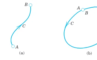
The curve Cis called the path of integration. Look at Fig. 219a. The path of integration goes from Ato B.Thus A: is its initial point and B: is its terminal point. Cis now oriented. The direction from A to B, in which t increases is called the positive direction on C. We mark it by an arrow. The points Aand Bmay coincide, as it happens in Fig. 219b. Then Cis called a closed path.

r(b) r(a)

(a⬉t⬉b). r(t)⫽_[x(t), y(t), z(t)]⫽x(t)i⫹y(t)j⫹z(t)k

C C

B

B

A

A

(a) (b)

Fig. 219. Oriented curve

Cis called a smooth curveif it has at each point a unique tangent whose direction varies continuously as we move along C. We note that r(t) in (2) is differentiable. Its derivative

is continuous and different from the zero vector at every point of C.

General Assumption

In this book, every path of integration of a line integral is assumed to be piecewise smooth, that is, it consists of finitely manysmooth curves.

For example, the boundary curve of a square is piecewise smooth. It consists of four smooth curves or, in this case, line segments which are the four sides of the square.

Definition and Evaluation of Line Integrals

A line integralof a vector function over a curve C: is defined by

(3)

where r(t) is the parametric representation of Cas given in (2). (The dot product was defined in Sec. 9.2.) Writing (3) in terms of components, with as in Sec. 9.5

and we get

⫽

冮

b

a

(F1x

r

⫹F2y

r

⫹F3z

r

) dt.

冮

C

F(r)•dr⫽

冮

C

(F1 dx⫹F2 dy⫹F3 dz) (3

r

)

r

⫽d>dt,

dr⫽_[dx, dy, dz]

r

_r

⫽ dr dt

冮

C

F(r)•dr⫽

冮

b

a

F(r(t))•r

r

(t) dt

r(t) F(r)

If the path of integration Cin (3) is a closedcurve, then instead of

we also write

Note that the integrand in (3) is a scalar, not a vector, because we take the dot product. Indeed, is the tangential component of F. (For “component” see (11) in Sec. 9.2.) We see that the integral in (3) on the right is a definite integral of a function of ttaken over the interval on the t-axis in the positive direction: The direction of increasing t. This definite integral exists for continuous Fand piecewise smooth C, because this makes piecewise continuous.

Line integrals (3) arise naturally in mechanics, where they give the work done by a force Fin a displacement along C.This will be explained in detail below. We may thus call the line integral (3) the work integral. Other forms of the line integral will be discussed later in this section.

E X A M P L E 1 Evaluation of a Line Integral in the Plane

Find the value of the line integral (3) when and Cis the circular arc in Fig. 220

from Ato B.

Solution. We may represent C by where Then and

By differentiation, so that by (3) [use (10) in App. 3.1; set

in the second term]

E X A M P L E 2 Line Integral in Space

The evaluation of line integrals in space is practically the same as it is in the plane. To see this, find the value

of (3) when and Cis the helix (Fig. 221)

(4) .

Solution. From (4) we have Thus

The dot product is Hence (3) gives

Simple general properties of the line integral (3)follow directly from corresponding properties of the definite integral in calculus, namely,

(5a)

冮

(kconstant)

Fig. 220. Example 1

z

x y

C B

A

(5b)

(5c) (Fig. 222)

where in (5c) the path C is subdivided into two arcs and that have the same orientation as C(Fig. 222). In (5b) the orientation of Cis the same in all three integrals. If the sense of integration along Cis reversed, the value of the integral is multiplied by⫺_1. However, we note the following independence if the sense is preserved.

T H E O R E M 1 Direction-Preserving Parametric Transformations

Any representations of C that give the same positive direction on C also yield the same value of the line integral (3).

P R O O F The proof follows by the chain rule. Let r(t) be the given representation with

as in (3). Consider the transformation which transforms the t interval to and has a positive derivative We write

Then and

Motivation of the Line Integral (3):

Work Done by a Force

The work Wdone by a constantforce Fin the displacement along a straightsegment d is ; see Example 2 in Sec. 9.2. This suggests that we define the work W done by a variableforce Fin the displacement along a curve C: as the limit of sums of works done in displacements along small chords of C. We show that this definition amounts to defining Wby the line integral (3).

For this we choose points Then the work done

by in the straight displacement from to is

The sum of these n works is If we choose points and

consider for every narbitrarily but so that the greatest approaches zero as then the limit of as is the line integral (3). This integral exists because of our general assumption that F is continuous and Cis piecewise smooth; this makes continuous, except at finitely many points where Cmay have corners

E X A M P L E 3 Work Done by a Variable Force

If Fin Example 1 is a force, the work done by Fin the displacement along the quarter-circle is 0.4521, measured

in suitable units, say, newton-meters (nt m, also called joules, abbreviation J; see also inside front cover). Similarly in Example 2.

E X A M P L E 4 Work Done Equals the Gain in Kinetic Energy

Let Fbe a force, so that (3) is work. Let tbe time, so that , velocity. Then we can write (3) as

(6)

Now by Newton’s second law, that is, , we get

where mis the mass of the body displaced. Substitution into (5) gives [see (11), Sec. 9.4]

On the right, is the kinetic energy. Hence the work done equals the gain in kinetic energy.This is a

basic law in mechanics.

Other Forms of Line Integrals

The line integrals

(7)

are special cases of (3) when or or , respectively.

Furthermore, without taking a dot product as in (3) we can obtain a line integral whose value is a vector rather than a scalar, namely,

(8)

Obviously, a special case of (7) is obtained by taking Then

(8*)

with Cas in (2). The evaluation is similar to that before.

E X A M P L E 5 A Line Integral of the Form (8)

Integrate along the helix in Example 2.

Solution. integrated with respect to tfrom 0 to gives

䊏

force⫽_mass⫻_acceleration

Path Dependence

Path dependence of line integrals is practically and theoretically so important that we formulate it as a theorem. And a whole section (Sec. 10.2) will be devoted to conditions under which path dependence does not occur.

T H E O R E M 2 Path Dependence

The line integral(3) generally depends not only onF and on the endpoints A and B of the path, but also on the path itself along which the integral is taken.

P R O O F Almost any example will show this. Take, for instance, the straight segment

and the parabola with (Fig. 223) and integrate

. Then so that integration gives

and 2>5,respectively. 䊏

1. WRITING PROJECT. From Definite Integrals to Line Integrals.Write a short report (1–2 pages) with examples on line integrals as generalizations of definite integrals. The latter give the area under a curve. Explain the corresponding geometric interpretation of a line integral.

2–11 LINE INTEGRAL. WORK

Calculate for the given data. If Fis a force, this

gives the work done by the force in the displacement along

C. Show the details.

2. from (0, 0) to (1, 4)

12. PROJECT. Change of Parameter. Path Dependence.

Consider the integral where

(a) One path, several representations. Find the value of the integral when

Show that the value remains the same if you set or or apply two other parametric transformations of your own choice.

(b) Several paths. Evaluate the integral when

thus where Note that these infinitely many paths have the same endpoints.

(c) Limit. What is the limit in (b) as ? Can you confirm your result by direct integration without referring to (b)?

(d) Show path dependence with a simple example of your choice involving two paths.

13. ML-Inequality, Estimation of Line Integrals.Let F be a vector function defined on a curve C. Let be bounded, say, on C, where Mis some positive number. Show that

(9)

14. Using (9), find a bound for the absolute value of the

work W done by the force in the

dis-placement from (0, 0) straight to (3, 4). Integrate exactly and compare.

18. the hypocycloid

19.

10.2

Path Independence of Line Integrals

We want to find out under what conditions, in some domain, a line integral takes on the same value no matter what path of integration is taken (in that domain). As before we consider line integrals

(1)

The line integral (1) is said to be path independent in a domain Din space if for every pair of endpoints A, Bin domain D, (1) has the same value for all paths in Dthat begin at Aand end at B. This is illustrated in Fig. 224. (See Sec. 9.6 for “domain.”)

Path independence is important. For instance, in mechanics it may mean that we have to do the same amount of work regardless of the path to the mountaintop, be it short and steep or long and gentle. Or it may mean that in releasing an elastic spring we get back the work done in expanding it. Not all forces are of this type—think of swimming in a big round pool in which the water is rotating as in a whirlpool.

We shall follow up with three ideas about path independence. We shall see that path independence of (1) in a domain Dholds if and only if:

(Theorem 1) where grad fis the gradient of fas explained in Sec. 9.7. (Theorem 2) Integration around closed curves Cin Dalways gives 0.

(Theorem 3) , provided Dis simply connected, as defined below.

Do you see that these theorems can help in understanding the examples and counterexample just mentioned?

T H E O R E M 1 Path Independence

A line integral (1) with continuous in a domain D in space is path independent in D if and only if is the gradient of some function f in D,

(2) thus,

P R O O F (a) We assume that (2) holds for some function f in Dand show that this implies path independence. Let Cbe any path in D from any point A to any point Bin D, given by , where . Then from (2), the chain rule in Sec. 9.6, and in the last section we obtain

(b) The more complicated proof of the converse, that path independence implies (2) for some f, is given in App. 4.

The last formula in part (a) of the proof,

(3)

is the analog of the usual formula for definite integrals in calculus,

Formula (3) should be applied whenever a line integral is independent of path.

Potential theoryrelates to our present discussion if we remember from Sec. 9.7 that when then fis called a potential of F. Thus the integral (1) is independent of path in Dif and only if Fis the gradient of a potential in D.

F_{grad f,}

[G

r

(x)_g(x)].

冮

b

a

g(x) dx_G(x)2 a b

_G(b)⫺G(a)

[F⫽_grad f ]

冮

B

A

(F1 dx⫹F2 dy⫹F3 dz)⫽f(B)⫺f(A)

䊏

⫽_f(B)⫺_f(A).

⫽_{f(x(b), y(b), z(b))}⫺_{f(x(a), y(a), z(a))} ⫽

冮

b

a df

dtdt⫽f[x(t), y(t), z(t)]2 t⫽_a

t⫽b ⫽

冮

b

a

a₀0_xf dx dt ⫹

0f

0y

dy dt ⫹

0f

0z

dz dtbdt

冮

C

(F1 dx⫹F2 dy⫹F3 dz)⫽

冮

C

a₀0_xf dx⫹ 0f

0ydy⫹

0f

0zdzb

(3

_r

)

a⬉t⬉b r(t)⫽_[x(t), y(t), z(t)]

F1⫽

0f

0x, F2⫽

0f

0y, F3⫽

0f

0z.

F⫽_grad f,

E X A M P L E 1 Path Independence

Show that the integral is path independent in any domain in space and

find its value in the integration from A: (0, 0, 0) to B: (2, 2, 2).

Solution. where because

Hence the integral is independent of path according to Theorem 1, and (3) gives

If you want to check this, use the most convenient path on which

so that and integration from 0 to 2 gives

If you did not see the potential by inspection, use the method in the next example.

E X A M P L E 2 Path Independence. Determination of a Potential

Evaluate the integral from to by showing that F has a

potential and applying (3).

Solution. If Fhas a potential f, we should have

We show that we can satisfy these conditions. By integration of fxand differentiation,

This gives and by (3),

Path Independence and Integration

Around Closed Curves

The simple idea is that two paths with common endpoints (Fig. 225) make up a single closed curve. This gives almost immediately

T H E O R E M 2 Path Independence

The integral(1) is path independent in a domain D if and only if its value around every closed path in D is zero.

P R O O F If we have path independence, then integration from A to B along and along in Fig. 225 gives the same value. Now and together make up a closed curve C, and if we integrate from Aalong to Bas before, but then in the opposite sense along back to A(so that this second integral is multiplied by ), the sum of the two integrals is zero, but this is the integral around the closed curve C.

Conversely, assume that the integral around any closed path Cin Dis zero. Given any points Aand Band any two curves and from Ato Bin D, we see that with the orientation reversed and together form a closed path C. By assumption, the integral over Cis zero. Hence the integrals over and , both taken from Ato B, must be equal.

This proves the theorem. 䊏

C2 C1 C2

C1 C2

C1

⫺₁

C2 C1

C2 C1

C2 C1

䊏

I⫽f(1, ⫺1, 7)⫺f(0, 1, 2)⫽1⫹7⫺(0⫹2)⫽6.

f(x,y,z)⫽x3_⫹y3_z

fz⫽y2⫹hr⫽y2, hr⫽0 h⫽0, say.

f⫽x3⫹g(y, z), fy⫽gy⫽2yz, g⫽y2z⫹h(z), f⫽x3⫹y2z⫹h(z)

fx⫽F1⫽3x

2_,

fy⫽F2⫽2yz, fz⫽F3⫽y

2_.

B: (1, ⫺_{1, 7)}

A: (0, 1, 2)

I⫽

冮

C

(3x2 dx⫹_2yzdy⫹_y2

dz)

䊏

8#22

>2⫽16.

F(r(t))•rr(t)⫽2t⫹2t⫹4t⫽8t,

F(r(t)⫽[2t, 2t, 4t],

C: r(t)⫽[t, t, t], 0⬉t⬉2,

f(B)⫺f(A)⫽f(2, 2, 2)⫺f(0, 0, 0)⫽4⫹4⫹8⫽16.

0f>0z⫽4z⫽F3.

0f>0y⫽2y⫽F2,

0f>0x⫽2x⫽F1,

f⫽x2⫹y2⫹2z2

F⫽[2x, 2y, 4z]⫽grad f,

冮

C

F•dr⫽

冮

C

(2xdx⫹₂ydy⫹₄zdz)

B

A C₁

C₂

Work. Conservative and Nonconservative (Dissipative) Physical Systems

Recall from the last section that in mechanics, the integral (1) gives the work done by a force Fin the displacement of a body along the curve C. Then Theorem 2 states that work is path independent in D if and only if its value is zero for displacement around every closed path in D. Furthermore, Theorem 1 tells us that this happens if and only if Fis the gradient of a potential in D. In this case, F and the vector field defined by F are called conservativein Dbecause in this case mechanical energy is conserved; that is, no work is done in the displacement from a point Aand back to A. Similarly for the displacement of an electrical charge (an electron, for instance) in a conservative electrostatic field.

Physically, the kinetic energy of a body can be interpreted as the ability of the body to do work by virtue of its motion, and if the body moves in a conservative field of force, after the completion of a round trip the body will return to its initial position with the same kinetic energy it had originally. For instance, the gravitational force is conservative; if we throw a ball vertically up, it will (if we assume air resistance to be negligible) return to our hand with the same kinetic energy it had when it left our hand.

Friction, air resistance, and water resistance always act against the direction of motion. They tend to diminish the total mechanical energy of a system, usually converting it into heat or mechanical energy of the surrounding medium (possibly both). Furthermore, if during the motion of a body, these forces become so large that they can no longer be neglected, then the resultant force F of the forces acting on the body is no longer conservative. This leads to the following terms. A physical system is called conservative if all the forces acting in it are conservative. If this does not hold, then the physical system is called nonconservativeor dissipative.

Path Independence and Exactness

of Differential Forms

Theorem 1 relates path independence of the line integral (1) to the gradient and Theorem 2 to integration around closed curves. A third idea (leading to Theorems and 3, below) relates path independence to the exactness of the differential formor Pfaffian form1

(4)

under the integral sign in (1). This form (4) is called exactin a domain Din space if it is the differential

of a differentiable function f(x, y, z) everywhere in D, that is, if we have

Comparing these two formulas, we see that the form (4) is exact if and only if there is a differentiable function f (x, y, z) in Dsuch that everywhere in D,

(5) thus, F1

0f

0x, F2

0f

0y, F3

0f

0z.

Fgrad _f,

F•drdf.

df

0f

0xdx

0f

0ydy

0f

0zdz(grad f )•dr F•drF1 dxF2 dyF3 dz

3*

Hence Theorem 1 implies

T H E O R E M 3 * Path Independence

The integral(1) is path independent in a domain D in space if and only if the differential form(4) has continuous coefficient functions and is exact in D.

This theorem is of practical importance because it leads to a useful exactness criterion. First we need the following concept, which is of general interest.

A domain Dis called simply connectedif every closed curve in Dcan be continuously shrunk to any point in Dwithout leaving D.

For example, the interior of a sphere or a cube, the interior of a sphere with finitely many points removed, and the domain between two concentric spheres are simply connected. On the other hand, the interior of a torus, which is a doughnut as shown in Fig. 249 in Sec. 10.6 is not simply connected. Neither is the interior of a cube with one space diagonal removed.

The criterion for exactness (and path independence by Theorem ) is now as follows.

T H E O R E M 3 Criterion for Exactness and Path Independence

Let in the line integral(1),

be continuous and have continuous first partial derivatives in a domain D in space. Then: (a) If the differential form (4) is exact in D—and thus (1)is path independent by Theorem —, then in D,

(6)

in components(see Sec. 9.9)

(b) If (6)holds in D and D is simply connected, then (4) is exact in D—and thus (1) is path independent by Theorem

P R O O F (a) If (4) is exact in D, then in D by Theorem and, furthermore, by (2) in Sec. 9.9, so that (6) holds.

(b) The proof needs “Stokes’s theorem” and will be given in Sec. 10.9.

Line Integral in the Plane. For the curl has only one

component (the z-component), so that reduces to the single relation

(which also occurs in (5) of Sec. 1.4 on exact ODEs).

0F2

0x

0F1

0y

(6

_s

)

(6

r

)

冮

C

F(r)•dr

冮

C

(F1 dxF2 dy)

䊏

curl Fcurl (grad f )₀

3*, Fgrad f

3*.

0F3

0y

0F2

0z ,

0F1

0z

0F3

0x ,

0F2

0x

0F1

0y .

(6

_r

)

curl F₀; 3*

冮

C

F(r)•dr

冮

C

(F1 dxF2 dyF3 dz), F1, F2, F3

E X A M P L E 3 Exactness and Independence of Path. Determination of a Potential

Using , show that the differential form under the integral sign of

is exact, so that we have independence of path in any domain, and find the value of Ifrom to

Solution. Exactness follows from which gives

To find f, we integrate (which is “long,” so that we save work) and then differentiate to compare with and

implies and we can take so that in the first line. This gives, by (3),

The assumption in Theorem 3 that Dis simply connected is essential and cannot be omitted. Perhaps the simplest example to see this is the following.

E X A M P L E 4 On the Assumption of Simple Connectedness in Theorem 3

Let

(7)

Differentiation shows that is satisfied in any domain of the xy-plane not containing the origin, for example,

in the domain shown in Fig. 226. Indeed, and do not depend on z, and ,

so that the first two relations in are trivially true, and the third is verified by differentiation:

Clearly, Din Fig. 226 is not simply connected. If the integral

were independent of path in D, then on any closed curve in D, for example, on the circle

But setting and noting that the circle is represented by , we have

x_{cos u,} dx sin udu, y_{sin u,} dy_{cos u}du,

r₁

x_{r cos u, yr sin u}

x2_y2_1.

I₀

I

冮

C

(F1 dxF2 dy)

冮

C

_ydxxdy

x2_y2

0F1

0y

x2_y2_y#_2y

(x2_y2₎2

y2_x2

(x2_y2₎2.

0F2

0x

x2_y2_x#_2x

(x2_y2₎2

y2_x2

(x2_y2₎2,

(6r)

F30

F2

F1

D: 1

22x

2

y23₂

(6r)

F1

y

x2_y2, F2

x

x2_y2, F3

_0.

䊏

f(x, y, z)x2_yz2_{sin yz, f(B)f(A)1}#p

4 #4sin

p

2 0p1.

g₀

h_0,

h_const

hr₀

fz2x2zyy cos yzhrF32x2zyy cos yz, hr0.

fx2xz2ygxF12xyz2, gx0, gh(z)

f

冮

F2 dy

冮

(x2z2z cos yz) dyx2z2ysin yzg(x, z)

F3,

F1

F2

(F2)x2xz2(F1)y.

(F1)z4xyz(F3)x

(F3)y2x2zcos yzyz sin yz(F2)z

(6r),

B: (1, p>4, 2).

A: (0, 0, 1)

I

冮

C

[2xyz2 _dx(x2_z2_{z cos yz) dy(2x}2_{yzy cos yz) dz]}

so that and counterclockwise integration gives

Since Dis not simply connected, we cannot apply Theorem 3 and cannot conclude that Iis independent of path

in D.

Although where (verify!), we cannot apply Theorem 1 either because the polar

angle f_{uarctan (}y>x)is not single-valued, as it is required for a function in calculus. 䊏

Fig. 226. Example 4

y

Project 10. Path Dependence 1. WRITING PROJECT. Report on Path Independence.

Make a list of the main ideas and facts on path independence and dependence in this section. Then work this list into a report. Explain the definitions and the practical usefulness of the theorems, with illustrative examples of your own. No proofs.

2. On Example 4. Does the situation in Example 4 of the text change if you take the domain

3–9 PATH INDEPENDENT INTEGRALS

Show that the form under the integral sign is exact in the plane (Probs. 3–4) or in space (Probs. 5–9) and evaluate the integral. Show the details of your work.

3.

10. PROJECT. Path Dependence. (a) Show that

is path dependent in the

xy-plane.

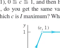
(b) Integrate from (0, 0) along the straight-line segment to (1, b), and then vertically up to (1, 1); see the figure. For which bis Imaximum? What is its maximum value?

(c) Integrate Ifrom (0, 0) along the straight-line segment to (c, 1), and then horizontally to (1, 1). For , do you get the same value as for in (b)? For which cis Imaximum? What is its maximum value?

10.3

Calculus Review: Double Integrals.

Optional

This section is optional. Students familiar with double integrals from calculus should skip this review and go on to Sec. 10.4. This section is included in the book to make it reasonably self-contained.

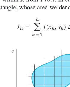
In a definite integral (1), Sec. 10.1, we integrate a function over an interval (a segment) of the x-axis. In a double integral we integrate a function , called the integrand,over a closed bounded region2Rin the xy-plane, whose boundary curve has a unique tangent at almost every point, but may perhaps have finitely many cusps (such as the vertices of a triangle or rectangle).

The definition of the double integral is quite similar to that of the definite integral. We subdivide the region Rby drawing parallels to the x- and y-axes (Fig. 227). We number the rectangles that are entirely within Rfrom 1 to n. In each such rectangle we choose a point, say, in the kth rectangle, whose area we denote by Then we form the sum

J_{n a}

n

k1

f(x_k, y_k) ¢A_k.

¢Ak.

(xk, yk)

f(x, y) f(x)

2_A

region Ris a domain (Sec. 9.6) plus, perhaps, some or all of its boundary points. Ris closedif its boundary

(all its boundary points) are regarded as belonging to R; and Ris boundedif it can be enclosed in a circle of

sufficiently large radius. A boundary pointPof Ris a point (of Ror not) such that every disk with center P

contains points of Rand also points not of R.

y

x

Fig. 227. Subdivision of a region R

11. On Example 4. Show that in Example 4 of the text, Give examples of domains in which the integral is path independent.

12. CAS EXPERIMENT. Extension of Project 10.

Inte-grate over various circles through the

points (0, 0) and (1, 1). Find experimentally the smallest value of the integral and the approximate location of the center of the circle.

13–19 PATH INDEPENDENCE?

Check, and if independent, integrate from (0, 0, 0) to (a, b,c). 13. 2ex2(x cos 2ydx⫺_{sin 2ydy)}

x2ydx⫹_2xy2 _dy F⫽grad (arctan ( y>x)).

14.

15.

16.

17.

18.

19.

20. Path Dependence. Construct three simple examples in each of which two equations are satisfied, but the third is not.

(6_r) (cos (x2⫹_2y2_⫹

z2)) (2xdx⫹_4ydy⫹_2zdz)

(cos xy)(yzdx⫹_xzdy)⫺_{2 sin xydz}

4ydx⫹zdy⫹( y⫺2z) dz eydx⫹(xey⫺ez) dy⫺yezdz x2ydx⫺4xy2 dy⫹8z2xdz

R₁

R₂

Fig. 228. Formula (1)

This we do for larger and larger positive integers nin a completely independent manner, but so that the length of the maximum diagonal of the rectangles approaches zero as n approaches infinity. In this fashion we obtain a sequence of real numbers

Assuming that is continuous in Rand Ris bounded by finitely many smooth curves (see Sec. 10.1), one can show (see Ref. [GenRef4] in App. 1) that this sequence converges and its limit is independent of the choice of subdivisions and corresponding points This limit is called the double integral of over the region R, and is denoted by

or

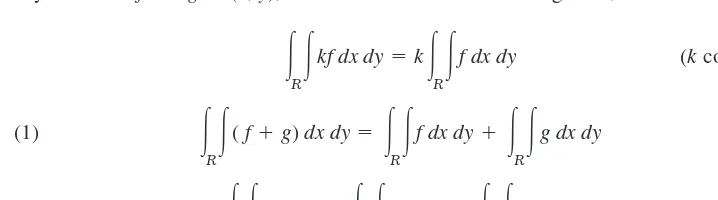
Double integrals have properties quite similar to those of definite integrals. Indeed, for any functions fand gof (x, y), defined and continuous in a region R,

(kconstant)

(1)

(Fig. 228).

Furthermore, if Ris simply connected (see Sec. 10.2), then there exists at least one point in Rsuch that we have

(2)

where Ais the area of R. This is called the mean value theoremfor double integrals.

冮

R

冮

f(x, y) dxdyf(x0, y0)A, (x0, y0)

冮

R

冮

fdxdy

冮

R1

冮

fdxdy

冮

R2

冮

fdxdy

冮

R

冮

( fg) dxdy

冮

R

冮

fdxdy

冮

R

冮

gdxdy

冮

R

冮

kfdxdyk

冮

R

冮

fdxdy

冮

R

冮

f(x, y) dA.

冮

R

冮

f(x, y) dxdy

f(x, y) (xk, yk).

f(x, y)

Jn1, Jn2,

Á_.

Evaluation of Double Integrals

by Two Successive Integrations

Double integrals over a region R may be evaluated by two successive integrations.We may integrate first over yand then over x. Then the formula is

(3)

冮

(Fig. 229).

R

冮

f(x, y) dxdy

冮

b

a

c

冮

h(x)

g(x)

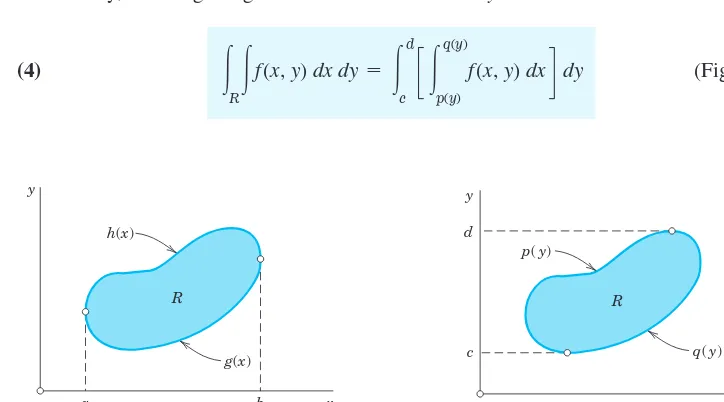
Here and represent the boundary curve of R(see Fig. 229) and, keeping xconstant, we integrate over yfrom to . The result is a function of x, and we integrate it from to (Fig. 229).

Similarly, for integrating first over xand then over ythe formula is

(4)

冮

(Fig. 230).

R

冮

f(x, y) dxdy

冮

d

c

c

冮

q(y)

p(y)

f(x, y) dxd dy x_b

x_a

h(x) g(x) f(x, y)

y_h(_x) y_g(_x)

y

x h(x)

g(x)

b a

R

y

x p(y)

q(y)

c d

R

Fig. 229. Evaluation of a double integral Fig. 230. Evaluation of a double integral

The boundary curve of R is now represented by and Treating yas a constant, we first integrate over xfrom to (see Fig. 230) and then the resulting function of yfrom to

In (3) we assumed that Rcan be given by inequalities and

Similarly in (4) by and If a region Rhas no such representation, then, in any practical case, it will at least be possible to subdivide Rinto finitely many portions each of which can be given by those inequalities. Then we integrate over each portion and take the sum of the results. This will give the value of the integral of

over the entire region R.

Applications of Double Integrals

Double integrals have various physical and geometric applications. For instance, the area Aof a region Rin the xy-plane is given by the double integral

The volumeVbeneath the surface and above a region Rin the xy-plane is (Fig. 231)

because the term in at the beginning of this section represents the volume of a rectangular box with base of area ¢Akand altitude f(xk, yk).

Jn f(xk, yk)¢Ak

V

冮

R

冮

f(x, y) dxdy z_{f(x, y) ( 0)}

A

冮

R

冮

dxdy. f(x, y)

f(x, y) p(y)⬉x⬉q(y).

c⬉y⬉d

g(x)⬉y⬉h(x). a⬉x⬉b

y⫽d. y⫽c

q(y) p(y) f(x, y)

As another application, let be the density ( mass per unit area) of a distribution of mass in the xy-plane. Then the total massMin Ris

the center of gravityof the mass in Rhas the coordinates , where

and

the moments of inertia and of the mass in Rabout the x- and y-axes, respectively, are

and the polar moment of inertia about the origin of the mass in Ris

An example is given below.

Change of Variables in Double Integrals. Jacobian

Practical problems often require a change of the variables of integration in double integrals. Recall from calculus that for a definite integral the formula for the change from xto uis

(5) .

Here we assume that is continuous and has a continuous derivative in some

interval such that and varies

between aand bwhen uvaries between and .

The formula for a change of variables in double integrals from x, yto u, vis

(6)

冮

R

冮

f(x, y) dxdy

冮

R*

冮

f(x(u, v), y(u, v)) 2 0(x, y)

0(u, v) 2 dudv;

b a

x(u) x(a)a, x(b)b[or x(a)b, x(b)a]

a⬉u⬉b

x⫽x(u)

冮

b

a

f(x) dx⫽

冮

b

a

f(x(u)) dx du du I0⫽Ix⫹Iy⫽

冮

R

冮

(x2⫹_y2_{)f(x, y) dxdy.} I0

Ix⫽

冮

R

冮

y2f(x, y) dxdy, Iy⫽

冮

R

冮

x2f(x, y) dxdy; Iy

Ix

y⫽ 1 M

冮

R

冮

yf(x, y) dxdy; x⫽ 1

M

冮

R

冮

xf(x, y) dxdy

x, y

M⫽

冮

R

冮

f(x, y) dxdy; ⫽ f(x, y)

z

x y

R

f(x, y)

that is, the integrand is expressed in terms of uand v, and dx dyis replaced by du dvtimes the absolute value of the Jacobian3

(7)

Here we assume the following. The functions

effecting the change are continuous and have continuous partial derivatives in some region in the uv-plane such that for every (u, v) in the corresponding point (x, y) lies in Rand, conversely, to every (x, y) in Rthere corresponds one and only one (u, v) in ; furthermore, the Jacobian Jis either positive throughout or negative throughout . For a proof, see Ref. [GenRef4] in App. 1.

E X A M P L E 1 Change of Variables in a Double Integral

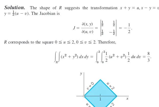
Evaluate the following double integral over the square Rin Fig. 232.

Solution. The shape of R suggests the transformation Then The Jacobian is

Rcorresponds to the square Therefore,

䊏

3_{Named after the German mathematician CARL GUSTAV JACOB JACOBI (1804–1851), known for his}

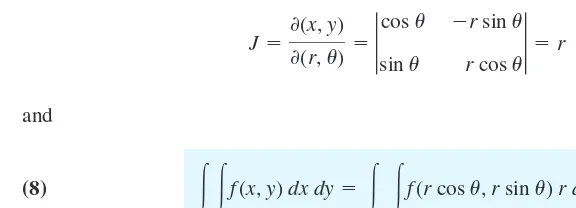
Of particular practical interest are polar coordinatesrand , which can be introduced

by setting Then

and

(8)

where is the region in the -plane corresponding to Rin the xy-plane.

E X A M P L E 2 Double Integrals in Polar Coordinates. Center of Gravity. Moments of Inertia

Let be the mass density in the region in Fig. 233. Find the total mass, the center of gravity, and the

moments of inertia

Solution. We use the polar coordinates just defined and formula (8). This gives the total mass

The center of gravity has the coordinates

for reasons of symmetry.

The moments of inertia are

for reasons of symmetry,

Why are and less than ?

This is the end of our review on double integrals. These integrals will be needed in this chapter, beginning in the next section.

1. Mean value theorem. Illustrate (2) with an example.

2–8 DOUBLE INTEGRALS

Describe the region of integration and evaluate.

2.

3.

4. Prob. 3, order reversed.

5.

6.

7. Prob. 6, order reversed.

8.

9–11 VOLUME

Find the volume of the given region in space.

9. The region beneath and above the

rectangle with vertices (0, 0), (3, 0), (3, 2), (0, 2) in the

xy-plane.

10. The first octant region bounded by the coordinate planes

and the surfaces Sketch it.

11. The region above the xy-plane and below the parabo-loid .

12–16 CENTER OF GRAVITY

Find the center of gravity of a mass of density in the given region R.

17–20 MOMENTS OF INERTIA

Find of a mass of density in the region

10.4

Green’s Theorem in the Plane

Double integrals over a plane region may be transformed into line integrals over the boundary of the region and conversely. This is of practical interest because it may simplify the evaluation of an integral. It also helps in theoretical work when we want to switch from one kind of integral to the other. The transformation can be done by the following theorem.

T H E O R E M 1 Green’s Theorem in the Plane4

(Transformation between Double Integrals and Line Integrals)

Let R be a closed bounded region(see Sec. 10.3) in the xy-plane whose boundary C consists of finitely many smooth curves(see Sec. 10.1). Let and be functions that are continuous and have continuous partial derivatives

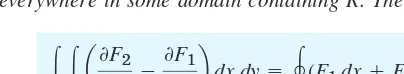
and everywhere in some domain containing R. Then

(1)

Here we integrate along the entire boundary C of R in such a sense that R is on the left as we advance in the direction of integration(see Fig. 234).

冮

R

冮

a0F2

0x ⫺

0F1

0y bdxdy⫽

冯

C

(F1 dx⫹F2 dy).

0F2>0x

0F1>0y

F2(x, y) F1(x, y)

4_{GEORGE GREEN (1793–1841), English mathematician who was self-educated, started out as a baker, and}

at his death was fellow of Caius College, Cambridge. His work concerned potential theory in connection with electricity and magnetism, vibrations, waves, and elasticity theory. It remained almost unknown, even in England, until after his death.

A “domain containing R” in the theorem guarantees that the assumptions about F1and F2at boundary points

of Rare the same as at other points of R.

y

x C₁ C₂

R

Fig. 234. Region Rwhose boundary Cconsists of two parts: is traversed counterclockwise, while is traversed clockwise

in such a way that Ris on the left for both curves

C2

C1

Setting and using (1)in Sec. 9.9, we obtain (1) in vectorial

form,

The proof follows after the first example. For 养see Sec. 10.1.

冮

R

冮

(curl F)•kdxdy⫽

冯

C F•dr.

(1

r

)

E X A M P L E 1 Verification of Green’s Theorem in the Plane

Green’s theorem in the plane will be quite important in our further work. Before proving it, let us get used to

it by verifying it for and Cthe circle

Solution. In (1) on the left we get

since the circular disk Rhas area

We now show that the line integral in (1) on the right gives the same value, We must orient C

counterclockwise, say, Then and on C,

Hence the line integral in (1) becomes, verifying Green’s theorem,

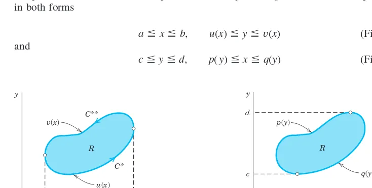
P R O O F We prove Green’s theorem in the plane, first for a special region Rthat can be represented in both forms

(Fig. 235) and

(Fig. 236) c⬉y⬉d, p(y)⬉x⬉q(y)

a⬉x⬉b, u(x)⬉y⬉_v(x)

䊏

⫽0⫹7p⫺0⫹2p⫽9p.

⫽

冮

2p

0

(⫺sin3

t⫹7 sin2

t⫹2 cos2

t sin t⫹2 cos2

t) dt

冯

_C(F1xr⫹F2 yr) dt⫽

冮

2p

0

[(sin2

t⫺_{7 sin t)(}⫺_{sin t)}⫹_{2(cos t sin t}⫹_{cos t)(cos t)] dt}

F1⫽y

2_⫺7

y⫽sin2

t⫺7 sin t, F2⫽2xy⫹2x⫽2 cos t sin t⫹2 cos t.

rr(t)⫽_[⫺_sin t, cos t],

r(t)⫽_[cos t, sin t].

9p.

p.

冮

R

冮

a0F2

0x ⫺

0F1

0ybdxdy⫽

冮

_R

冮

[(2y⫹2)⫺(2y⫺7)]dxdy⫽9

冮

_R

冮

dxdy⫽9p

x2_⫹y2_⫽1.

F1⫽y2⫺7y, F2⫽2xy⫹2x

y

x v(x)

u(x)

b a

R C**

C*

y

x p(y)

q(y)

c d

R

Fig. 235. Example of a special region Fig. 236. Example of a special region

Using (3) in the last section, we obtain for the second term on the left side of (1) taken without the minus sign

(2)

冮

(see Fig. 235).

R

冮

0F1

0y dxdy⫽

冮

b

a

c

冮

v(x)

u(x)

0F1

(The first term will be considered later.) We integrate the inner integral:

By inserting this into (2) we find (changing a direction of integration)

Since represents the curve (Fig. 235) and represents the last two integrals may be written as line integrals over and (oriented as in Fig. 235); therefore,

(3)

This proves (1) in Green’s theorem if .

The result remains valid if C has portions parallel to the y-axis (such as and in Fig. 237). Indeed, the integrals over these portions are zero because in (3) on the right we integrate with respect to x. Hence we may add these integrals to the integrals over and

to obtain the integral over the whole boundary Cin (3).

We now treat the first term in (1) on the left in the same way. Instead of (3) in the last section we use (4), and the second representation of the special region (see Fig. 236). Then (again changing a direction of integration)

Together with (3) this gives (1) and proves Green’s theorem for special regions. We now prove the theorem for a region Rthat itself is not a special region but can be subdivided into finitely many special regions as shown in Fig. 238. In this case we apply the theorem to each subregion and then add the results; the left-hand members add up to the integral over Rwhile the right-hand members add up to the line integral over Cplus

integrals over the curves introduced for subdividing R. The simple key observationnow is that each of the latter integrals occurs twice, taken once in each direction. Hence they cancel each other, leaving us with the line integral over C.

The proof thus far covers all regions that are of interest in practical problems. To prove the theorem for a most general region Rsatisfying the conditions in the theorem, we must approximate R by a region of the type just considered and then use a limiting process. For details of this see Ref. [GenRef4] in App. 1.

Some Applications of Green’s Theorem

E X A M P L E 2 Area of a Plane Region as a Line Integral Over the Boundary

In (1) we first choose and then This gives

respectively. The double integral is the area Aof R. By addition we have

(4)

where we integrate as indicated in Green’s theorem. This interesting formula expresses the area of Rin terms

of a line integral over the boundary. It is used, for instance, in the theory of certain planimeters(mechanical

instruments for measuring area). See also Prob. 11.

For an ellipse or we get thus from

(4) we obtain the familiar formula for the area of the region bounded by an ellipse,

E X A M P L E 3 Area of a Plane Region in Polar Coordinates

Let rand be polar coordinates defined by Then

dx_{cos udr}⫺r sin udu, dy⫽sin udr⫹r cos udu,

x⫽r cos u, y⫽r sin u.

u

䊏

A⫽1

2

冮

2p

0

(xyr⫺yxr) dt⫽1

2

冮

2p

0

[ab cos2

t⫺(⫺ab sin2

t)] dt⫽pab.

xr⫽ ⫺a sin t, yr⫽b cos t;

x⫽a cos t, y⫽b sin t

x2

>a2_⫹y2 >b2_⫽1

A⫽1

2

冯

C

(xdy⫺ydx)

冮

R

冮

dxdy⫽

冯

C

xdy and

冮

R

冮

dxdy⫽ ⫺

冯

C

ydx

F1⫽ ⫺y, F2⫽0.

F2⫽x

F1⫽0,

C**

C* C C

y

x

y

x

and (4) becomes a formula that is well known from calculus, namely,

(5)

As an application of (5), we consider the cardioid where (Fig. 239). We find

E X A M P L E 4 Transformation of a Double Integral of the Laplacian of a Function into a Line Integral of Its Normal Derivative

The Laplacian plays an important role in physics and engineering. A first impression of this was obtained in Sec. 9.7, and we shall discuss this further in Chap. 12. At present, let us use Green’s theorem for deriving a basic integral formula involving the Laplacian.

We take a function that is continuous and has continuous first and second partial derivatives in a

domain of the xy-plane containing a region Rof the type indicated in Green’s theorem. We set

and Then and are continuous in R, and in (1) on the left we obtain

(6)

the Laplacian of w(see Sec. 9.7). Furthermore, using those expressions for and we get in (1) on the right

(7)

where sis the arc length of C, and Cis oriented as shown in Fig. 240. The integrand of the last integral may

be written as the dot product

(8)

The vector nis a unit normal vector to C, because the vector is the unit tangent

vector of C, and , so that nis perpendicular to . Also, nis directed to the exteriorof Cbecause in

Fig. 240 the positive x-component of is the negative y-component of n, and similarly at other points. From

this and (4) in Sec. 9.7 we see that the left side of (8) is the derivative of win the direction of the outward normal

of C. This derivative is called the normal derivativeof wand is denoted by ; that is,

Because of (6), (7), and (8), Green’s theorem gives the desired formula relating the Laplacian to the normal derivative,

(9)

For instance, satisfies Laplace’s equation Hence its normal derivative integrated over a closed

curve must give 0. Can you verify this directly by integration, say, for the square 0⬉_x⬉_{1, 0}⬉_y⬉_{1? 䊏}

Green’s theorem in the plane can be used in both directions, and thus may aid in the evaluation of a given integral by transforming the given integral into another integral that is easier to solve. This is illustrated further in the problem set. Moreover, and perhaps more fundamentally, Green’s theorem will be the essential tool in the proof of a very important integral theorem, namely, Stokes’s theorem in Sec. 10.9.

1–10 LINE INTEGRALS: EVALUATION BY GREEN’S THEOREM

Evaluate counterclockwise around the boundary

Cof the region R by Green’s theorem, where

1. Cthe circle

2. R the square with vertices

3. Rthe rectangle with vertices (0, 0),

(2, 0), (2, 3), (0, 3)

4.

5.

6.

7. Ras in Prob. 5

8. Rthe semidisk

9.

10.

Sketch R.

11. CAS EXPERIMENT. Apply (4) to figures of your choice whose area can also be obtained by another method and compare the results.

12. PROJECT. Other Forms of Green’s Theorem in the Plane. Let Rand Cbe as in Green’s theorem, a unit tangent vector, and nthe outer unit normal vector of C(Fig. 240 in Example 4). Show that (1) may be

where kis a unit vector perpendicular to the xy-plane. Verify(10) and (11) for and Cthe circle as well as for an example of your own choice.

13–17 INTEGRAL

OF THE NORMAL DERIVATIVE

Using (9), find the value of dstaken counterclockwise over the boundary Cof the region R.

13. Rthe triangle with vertices (0, 0), (4, 2), (0, 2).

14.

15.

16. Confirm the answer

by direct integration.

17.

18. Laplace’s equation.Show that for a solution w(x, y) of Laplace’s equation in a region R with boundary curve Cand outer unit normal vector n,

(12)

19. Show that satisfies Laplace’s equation

and, using (12), integrate counter-clockwise around the boundary curve Cof the rectangle

20. Same task as in Prob. 19 when and C

10.5

Surfaces for Surface Integrals

Whereas, with line integrals, we integrate over curves in space (Secs. 10.1, 10.2), with surface integrals we integrate over surfaces in space. Each curve in space is represented by a parametric equation (Secs. 9.5, 10.1). This suggests that we should also find parametric representations for the surfaces in space. This is indeed one of the goals of this section. The surfaces considered are cylinders, spheres, cones, and others. The second goal is to learn about surface normals. Both goals prepare us for Sec. 10.6 on surface integrals. Note that for simplicity, we shall say “surface” also for a portion of a surface.

Representation of Surfaces

Representations of a surface Sin xyz-space are

(1)

For example, or represents a

hemisphere of radius aand center 0.

Now for curves Cin line integrals, it was more practical and gave greater flexibility to use a parametric representation where This is a mapping of the interval located on the t-axis, onto the curve C (actually a portion of it) in xyz-space. It maps every t in that interval onto the point of C with position vector See Fig. 241A.

Similarly, for surfaces Sin surface integrals, it will often be more practical to use a parametricrepresentation. Surfaces are two-dimensional. Hence we need twoparameters, r(t). a⬉t⬉b,

a⬉t⬉b. r⫽_r(t),

x2⫹y2⫹z2⫺a2⫽_{0 (}z⭌₀₎ z⫽ ⫹2a2⫺x2⫺y2

z⫽f(x, y) or g(x, y, z)⫽_0.

z

y x

r(t)

r(u,v)

Curve C

in space

z y x

a b

t

(t-axis)

v

u

R

(uv-plane)

Surface S

in space

(A) Curve (B) Surface

which we call uand v. Thus a parametric representationof a surface Sin space is of the form

(2)

where (u, v) varies in some region Rof the uv-plane. This mapping (2) maps every point (u, v) in Ronto the point of Swith position vector r(u, v). See Fig. 241B.

E X A M P L E 1 Parametric Representation of a Cylinder

The circular cylinder has radius a, height 2, and the z-axis as axis. A parametric

representation is

(Fig. 242).

The components of rare The parameters u, vvary in the rectangle

in the uv-plane. The curves are vertical straight lines. The curves are

parallel circles. The point Pin Fig. 242 corresponds to u_p>360°, v_0.7. 䊏

v_const

u_const

2p, ⫺₁⬉v⬉₁

R: 0⬉u⬉

x⫽a cos u, y⫽a sin u, z⫽v.

r(u, v)⫽[a cos u, a sin u, v]⫽a cos ui⫹a sin uj⫹vk

x2⫹y2⫽a2, ⫺₁⬉z⬉_1,

r(u, v)⫽_[x(u, v), y(u, v), z(u, v)]⫽x(u, v)i⫹y(u, v)j⫹z(u, v)k

(v= 1)

(v= 0)

(v= –1)

v u

P

y x

z

u v

P z

y x

Fig. 242. Parametric representation Fig. 243. Parametric representation

of a cylinder of a sphere

E X A M P L E 2 Parametric Representation of a Sphere

A sphere can be represented in the form

(3)

where the parameters u, v vary in the rectangle Rin the uv-plane given by the inequalities

The components of rare

The curves and are the “meridians” and “parallels” on S(see Fig. 243). This representation

is used ingeographyfor measuring the latitude and longitude of points on the globe.

Another parametric representation of the sphere also used in mathematics is

(3*)

where 0⬉u⬉2p, 0⬉v⬉p. _䊏

r(u, v)⫽a cos u sin vi⫹a sin u sin vj⫹a cos vk

v⫽const

u⫽const

x⫽a cos v cos u, y⫽a cos v sin u, z⫽a sin v.

⫺p>2⬉v⬉p>2.

0⬉u⬉2p,

r(u, v)⫽a cos v cos ui⫹a cos v sin uj⫹a sin vk

E X A M P L E 3 Parametric Representation of a Cone

A circular cone can be represented by

in components The parameters vary in the rectangle

Check that as it should be. What are the curves and ?

Tangent Plane and Surface Normal

Recall from Sec. 9.7 that the tangent vectors of all the curves on a surface Sthrough a point Pof Sform a plane, called the tangent planeof Sat P(Fig. 244). Exceptions are points where Shas an edge or a cusp (like a cone), so that Scannot have a tangent plane at such a point. Furthermore, a vector perpendicular to the tangent plane is called a normal vectorof Sat P. Now since Scan be given by in (2), the new idea is that we get a curve C on Sby taking a pair of differentiable functions

whose derivatives and are continuous. Then C has the position vector . By differentiation and the use of the chain rule (Sec. 9.6) we obtain a tangent vector of Con S

Hence the partial derivatives and at P are tangential to S at P.We assume that they are linearly independent, which geometrically means that the curves and on Sintersect at Pat a nonzero angle. Then and span the tangent plane of Sat P. Hence their cross product gives a normal vector Nof Sat P.

(4)

The corresponding unit normal vector nof Sat Pis (Fig. 244)

(5) n 1

ƒNƒ N

1

ƒruⴛrvƒ

ruⴛrv.

N_ruⴛrv0.

rv

ru vconst

uconst rv

ru r

~

_r

_(t) d~r

dt

0r

0uu

r

0r

0v

v

r

. r

~(t)_r(u(t), v(t))

v

r

dv>dt u

_r

du>dt

uu(t), vv(t) r_r(u, v)

䊏

v_const

u_const

x2_y2_z2_,

R: 0uH, 0v_2p.

xu cos v, yu sin v, zu.

r(u, v)[u cos v, u sin v, u]u cos viu sin vjuk,

z2x2_y2_{, 0tH}

n

r

v

r

u

P

S