Digital Speech
Digital Speech
Coding for Low Bit Rate Communication Systems
Second Edition
A. M. Kondoz
Copyright2004 John Wiley & Sons Ltd, The Atrium, Southern Gate, Chichester,
West Sussex PO19 8SQ, England
Telephone (+44) 1243 779777
Email (for orders and customer service enquiries): [email protected] Visit our Home Page on www.wileyeurope.com or www.wiley.com
All Rights Reserved. No part of this publication may be reproduced, stored in a retrieval system or transmitted in any form or by any means, electronic, mechanical, photocopying, recording, scanning or otherwise, except under the terms of the Copyright, Designs and Patents Act 1988 or under the terms of a licence issued by the Copyright Licensing Agency Ltd, 90 Tottenham Court Road, London W1T 4LP, UK, without the permission in writing of the Publisher. Requests to the Publisher should be addressed to the Permissions Department, John Wiley & Sons Ltd, The Atrium, Southern Gate, Chichester, West Sussex PO19 8SQ, England, or emailed to [email protected], or faxed to (+44) 1243 770620.
This publication is designed to provide accurate and authoritative information in regard to the subject matter covered. It is sold on the understanding that the Publisher is not engaged in rendering professional services. If professional advice or other expert assistance is required, the services of a competent professional should be sought.
Other Wiley Editorial Offices
John Wiley & Sons Inc., 111 River Street, Hoboken, NJ 07030, USA
Jossey-Bass, 989 Market Street, San Francisco, CA 94103-1741, USA
Wiley-VCH Verlag GmbH, Boschstr. 12, D-69469 Weinheim, Germany
John Wiley & Sons Australia Ltd, 33 Park Road, Milton, Queensland 4064, Australia
John Wiley & Sons (Asia) Pte Ltd, 2 Clementi Loop #02-01, Jin Xing Distripark, Singapore 129809
John Wiley & Sons Canada Ltd, 22 Worcester Road, Etobicoke, Ontario, Canada M9W 1L1
Wiley also publishes its books in a variety of electronic formats. Some content that appears in print may not be available in electronic books.
British Library Cataloguing in Publication Data
A catalogue record for this book is available from the British Library
ISBN 0-470-87007-9 (HB)
Typeset in 11/13pt Palatino by Laserwords Private Limited, Chennai, India Printed and bound in Great Britain by Antony Rowe Ltd, Chippenham, Wiltshire
Contents
Preface xiii
Acknowledgements xv
1 Introduction 1
2 Coding Strategies and Standards 5
2.1 Introduction 5
2.2 Speech Coding Techniques 6
2.2.1 Parametric Coders 7
2.2.2 Waveform-approximating Coders 8
2.2.3 Hybrid Coding of Speech 8
2.3 Algorithm Objectives and Requirements 9
2.3.1 Quality and Capacity 9
2.3.2 Coding Delay 10
2.3.3 Channel and Background Noise Robustness 10
2.3.4 Complexity and Cost 11
2.3.5 Tandem Connection and Transcoding 11
2.3.6 Voiceband Data Handling 11
2.4 Standard Speech Coders 12
2.4.1 ITU-T Speech Coding Standard 12
2.4.2 European Digital Cellular Telephony Standards 13 2.4.3 North American Digital Cellular Telephony Standards 14
2.4.4 Secure Communication Telephony 14
2.4.5 Satellite Telephony 15
2.4.6 Selection of a Speech Coder 15
2.5 Summary 18
Bibliography 18
3 Sampling and Quantization 23
3.2 Sampling 23
3.3 Scalar Quantization 26
3.3.1 Quantization Error 27
3.3.2 Uniform Quantizer 28
3.3.3 Optimum Quantizer 29
3.3.4 Logarithmic Quantizer 32
3.3.5 Adaptive Quantizer 33
3.3.6 Differential Quantizer 36
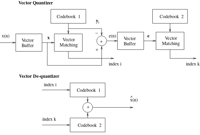
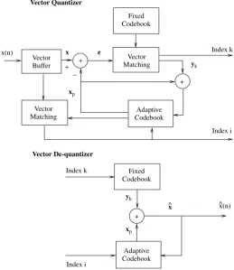
3.4 Vector Quantization 39
3.4.1 Distortion Measures 42
3.4.2 Codebook Design 43
3.4.3 Codebook Types 44
3.4.4 Training, Testing and Codebook Robustness 52
3.5 Summary 54
Bibliography 54
4 Speech Signal Analysis and Modelling 57
4.1 Introduction 57
4.2 Short-Time Spectral Analysis 57
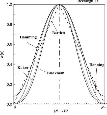
4.2.1 Role of Windows 58
4.3 Linear Predictive Modelling of Speech Signals 65
4.3.1 Source Filter Model of Speech Production 65
4.3.2 Solutions to LPC Analysis 67
4.3.3 Practical Implementation of the LPC Analysis 74
4.4 Pitch Prediction 77
4.4.1 Periodicity in Speech Signals 77
4.4.2 Pitch Predictor (Filter) Formulation 78
4.5 Summary 84
Bibliography 84
5 Efficient LPC Quantization Methods 87
5.1 Introduction 87
5.2 Alternative Representation of LPC 87
5.3 LPC to LSF Transformation 90
5.3.1 Complex Root Method 95
5.3.2 Real Root Method 95
5.3.3 Ratio Filter Method 98
5.3.4 Chebyshev Series Method 100
5.3.5 Adaptive Sequential LMS Method 100
Contents ix
5.4.1 Direct Expansion Method 101
5.4.2 LPC Synthesis Filter Method 102
5.5 Properties of LSFs 103
5.6 LSF Quantization 105
5.6.1 Distortion Measures 106
5.6.2 Spectral Distortion 106
5.6.3 Average Spectral Distortion and Outliers 107
5.6.4 MSE Weighting Techniques 107
5.7 Codebook Structures 110
5.7.1 Split Vector Quantization 111
5.7.2 Multi-Stage Vector Quantization 113
5.7.3 Search strategies for MSVQ 114
5.7.4 MSVQ Codebook Training 116
5.8 MSVQ Performance Analysis 117
5.8.1 Codebook Structures 117
5.8.2 Search Techniques 117
5.8.3 Perceptual Weighting Techniques 119
5.9 Inter-frame Correlation 121
5.9.1 LSF Prediction 122
5.9.2 Prediction Order 124
5.9.3 Prediction Factor Estimation 125
5.9.4 Performance Evaluation of MA Prediction 126
5.9.5 Joint Quantization of LSFs 128
5.9.6 Use of MA Prediction in Joint Quantization 129
5.10 Improved LSF Estimation Through Anti-Aliasing Filtering 130
5.10.1 LSF Extraction 131
5.10.2 Advantages of Low-pass Filtering in Moving Average
Prediction 135
5.11 Summary 146
Bibliography 146
6 Pitch Estimation and Voiced–Unvoiced Classification of Speech 149
6.1 Introduction 149
6.2 Pitch Estimation Methods 150
6.2.1 Time-Domain PDAs 151
6.2.2 Frequency-Domain PDAs 155
6.2.3 Time- and Frequency-Domain PDAs 158
6.2.4 Pre- and Post-processing Techniques 166
6.3 Voiced–Unvoiced Classification 178
6.3.1 Hard-Decision Voicing 178
6.4 Summary 196
Bibliography 197
7 Analysis by Synthesis LPC Coding 199
7.1 Introduction 199
7.2 Generalized AbS Coding 200
7.2.1 Time-Varying Filters 202
7.2.2 Perceptually-based Minimization Procedure 203
7.2.3 Excitation Signal 206
7.2.4 Determination of Optimum Excitation Sequence 208 7.2.5 Characteristics of AbS-LPC Schemes 212
7.3 Code-Excited Linear Predictive Coding 219
7.3.1 LPC Prediction 221
7.3.2 Pitch Prediction 222
7.3.3 Multi-Pulse Excitation 230
7.3.4 Codebook Excitation 238
7.3.5 Joint LTP and Codebook Excitation Computation 252
7.3.6 CELP with Post-Filtering 255
7.4 Summary 258
Bibliography 258
8 Harmonic Speech Coding 261
8.1 Introduction 261
8.2 Sinusoidal Analysis and Synthesis 262
8.3 Parameter Estimation 263
8.3.1 Voicing Determination 264
8.3.2 Harmonic Amplitude Estimation 266
8.4 Common Harmonic Coders 268
8.4.1 Sinusoidal Transform Coding 268
8.4.2 Improved Multi-Band Excitation, INMARSAT-M Version 270 8.4.3 Split-Band Linear Predictive Coding 271
8.5 Summary 275
Bibliography 275
9 Multimode Speech Coding 277
9.1 Introduction 277
9.2 Design Challenges of a Hybrid Coder 280
9.2.1 Reliable Speech Classification 281
9.2.2 Phase Synchronization 281
9.3 Summary of Hybrid Coders 281
Contents xi
9.3.2 Combined Harmonic and Waveform Coding at Low Bit-Rates 282
9.3.3 A 4 kb/s Hybrid MELP/CELP Coder 283
9.3.4 Limitations of Existing Hybrid Coders 284
9.4 Synchronized Waveform-Matched Phase Model 285
9.4.1 Extraction of the Pitch Pulse Location 286 9.4.2 Estimation of the Pitch Pulse Shape 292 9.4.3 Synthesis using Generalized Cubic Phase Interpolation 297
9.5 Hybrid Encoder 298
9.5.1 Synchronized Harmonic Excitation 299
9.5.2 Advantages and Disadvantages of SWPM 301
9.5.3 Offset Target Modification 304
9.5.4 Onset Harmonic Memory Initialization 308
9.5.5 White Noise Excitation 309
9.6 Speech Classification 311
9.6.1 Open-Loop Initial Classification 312
9.6.2 Closed-Loop Transition Detection 315
9.6.3 Plosive Detection 318
9.7 Hybrid Decoder 319
9.8 Performance Evaluation 320
9.9 Quantization Issues of Hybrid Coder Parameters 322
9.9.1 Introduction 322
9.9.2 Unvoiced Excitation Quantization 323
9.9.3 Harmonic Excitation Quantization 323
9.9.4 Quantization of ACELP Excitation at Transitions 331
9.10 Variable Bit Rate Coding 331
9.10.1 Transition Quantization with 4 kb/s ACELP 332 9.10.2 Transition Quantization with 6 kb/s ACELP 332 9.10.3 Transition Quantization with 8 kb/s ACELP 333
9.10.4 Comparison 334
9.11 Acoustic Noise and Channel Error Performance 336
9.11.1 Performance under Acoustic Noise 337
9.11.2 Performance under Channel Errors 345
9.11.3 Performance Improvement under Channel Errors 349
9.12 Summary 350
Bibliography 351
10 Voice Activity Detection 357
10.1 Introduction 357
10.2 Standard VAD Methods 360
10.2.2 ETSI GSM-FR/HR/EFR VAD 361
10.2.3 ETSI AMR VAD 362
10.2.4 TIA/EIA IS-127/733 VAD 363
10.2.5 Performance Comparison of VADs 364
10.3 Likelihood-Ratio-Based VAD 368
10.3.1 Analysis and Improvement of the Likelihood Ratio Method 370
10.3.2 Noise Estimation Based on SLR 373
10.3.3 Comparison 373
10.4 Summary 375
Bibliography 375
11 Speech Enhancement 379
11.1 Introduction 379
11.2 Review of STSA-based Speech Enhancement 381
11.2.1 Spectral Subtraction 382
11.2.2 Maximum-likelihood Spectral Amplitude Estimation 384
11.2.3 Wiener Filtering 385
11.2.4 MMSE Spectral Amplitude Estimation 386 11.2.5 Spectral Estimation Based on the Uncertainty of Speech
Presence 387
11.2.6 Comparisons 389
11.2.7 Discussion 392
11.3 Noise Adaptation 402
11.3.1 Hard Decision-based Noise Adaptation 402 11.3.2 Soft Decision-based Noise Adaptation 403 11.3.3 Mixed Decision-based Noise Adaptation 403
11.3.4 Comparisons 404
11.4 Echo Cancellation 406
11.4.1 Digital Echo Canceller Set-up 411
11.4.2 Echo Cancellation Formulation 413
11.4.3 Improved Performance Echo Cancellation 415
11.5 Summary 423
Bibliography 426
Preface
Speech has remained the most desirable medium of communication between humans. Nevertheless, analogue telecommunication of speech is a cumber-some and inflexible process when transmission power and spectral utilization, the foremost resources in any communication system, are considered. Dig-ital transmission of speech is more versatile, providing the opportunity of achieving lower costs, consistent quality, security and spectral efficiency in the systems that exploit it. The first stage in the digitization of speech involves sampling and quantizations. While the minimum sampling frequency is lim-ited by the Nyquist criterion, the number of quantifier levels is generally determined by the degree of faithful reconstruction (quality) of the signal required at the receiver. For speech transmission systems, these two limita-tions lead to an initial bit rate of 64 kb/s – the PCM system. Such a high bit rate restricts the much desired spectral efficiency.
The last decade has witnessed the emergence of new fixed and mobile telecommunication systems for which spectral efficiency is a prime mover. This has fuelled the need to reduce the PCM bit rate of speech signals. Digital coding of speech and the bit rate reduction process has thus emerged as an important area of research. This research largely addresses the following problems:
• Although it is very attractive to reduce the PCM bit rate as much as
possible, it becomes increasingly difficult to maintain acceptable speech quality as the bit rate falls.
• As the bit rate falls, acceptable speech quality can only be maintained by
employing very complex algorithms, which are difficult to implement in real-time even with new fast processors with their associated high cost and power consumption, or by incurring excessive delay, which may create echo control problems elsewhere in the system.
• In order to achieve low bit rates, parameters of a speech production and/or
on highly degraded channels, raising the acute problem of maintaining acceptable speech quality from sensitive speech parameters even in bad channel conditions. Moreover, when estimating these parameters from the input, speech contaminated by the environmental noise typical of mobile/wireless communication systems can cause significant degradation of speech quality.
These problems are by no means insurmountable. The advent of faster and more reliable Digital Signal Processor (DSP) chips has made possible the easy real-time implementation of highly complex algorithms. Their sophistication is also exploited in the implementation of more effective echo control, back-ground noise suppression, equalization and forward error control systems. The design of an optimum system is thus mainly a trading-off process of many factors which affect the overall quality of service provided at a reasonable cost.
This book presents some existing chapters from the first edition, as well as chapters on new speech processing and coding techniques. In order to lay the foundation of speech coding technology, it reviews sampling, quantizations and then the basic nature of speech signals, and the theory and tools applied in speech coding. The rest of the material presented has been drawn from recent postgraduate research and graduate teaching activities within the Multimedia Communications Research Group of the Centre for Communication Systems Research (CCSR), a teaching and research centre at the University of Surrey. Most of the material thus represents state-of-the-art thinking in this technology. It is suitable for both graduate and postgraduate teaching. It is hoped that the book will also be useful to research and development engineers for whom the hands-on approach to the base band design of low bit-rate fixed and mobile communication systems will prove attractive.
Acknowledgements
1
Introduction
Although data links are increasing in bandwidth and are becoming faster, speech communication is still the most dominant and common service in telecommunication networks. The fact that commercial and private usage of telephony in its various forms (especially wireless) continues to grow even a century after its first inception is obvious proof of its popularity as a form of communication. This popularity is expected to remain steady for the fore-seeable future. The traditional plain analogue system has served telephony systems remarkably well considering its technological simplicity. However, modern information technology requirements have introduced the need for a more robust and flexible alternative to the analogue systems. Although the encoding of speech other than straight conversion to an analogue signal has been studied and employed for decades, it is only in the last 20 to 30 years that it has really taken on significant prominence. This is a direct result of many factors, including the introduction of many new application areas.
The attractions of digitally-encoded speech are obvious. As speech is con-densed to a binary sequence, all of the advantages offered by digital systems are available for exploitation. These include the ease of regeneration and signalling, flexibility, security, and integration into the evolving new wire-less systems. Although digitally-encoded speech possesses many advantages over its analogue counterpart, it nevertheless requires extra bandwidth for transmission if it is directly applied (without compression). The 64 kb/s Log-PCM and 32 kb/s ADPCM systems which have served the many early generations of digital systems well over the years have therefore been found to be inadequate in terms of spectrum efficiency when applied to the new, bandwidth limited, communication systems, e.g. satellite communications, digital mobile radio systems, and private networks. In these and other sys-tems, the bandwidth and power available is severely restricted, hence signal compression is vital. For digitized speech, the signal compression is achieved via elaborate digital signal p rocessing techniques that are f acilitated by the
2 Introduction
rapid improvement in digital hardware which has enabled the use of sophis-ticated digital signal processing techniques that were not feasible before. In response to the requirement for speech compression, feverish research activ-ity has been pursued in all of the main research centres and, as a result, many different strategies have been developed for suitably compressing speech for bandwidth-restricted applications. During the last two decades, these efforts have begun to bear fruit. The use of low bit-rate speech coders has been standardized in many international, continental and national communication systems. In addition, there are a number of private network operators who use low bit-rate speech coders for specific applications.
The speech coding technology has gone through a number of phases starting with the development and deployment of PCM and ADPCM systems. This was followed by the development of good quality medium to low bit-rate coders covering the range from 16 kb/s to 8 kb/s. At the same time, very low bit-rate coders operating at around 2.4 kb/s produced better quality synthetic speech at the expense of higher complexity. The latest trend in speech coding is targeting the range from about 6 kb/s down to 2 kb/s by using specific coders, which rely heavily on the extraction of speech-specific information from the input source. However, as the main applications of the low to very low bit-rate coders are in the area of mobile communication systems, where there may be significant levels of background noise, the accurate determination of the speech parameters becomes more difficult. Therefore the use of active noise suppression as a preprocessor to low bit-rate speech coding is becoming popular.
In addition to the required low bit-rate for spectral efficiency, the cost and power requirements of speech encoder/decoder hardware are very important. In wireless personal communication systems, where hand-held telephones are used, the battery consumption, cost and size of the portable equipment have to be reasonable in order to make the product widely acceptable.
In this book an attempt is made to cover many important aspects of low bit-rate speech coding. In Chapter 2, the background to speech coding, including the existing standards, is discussed. In Chapter 3, after briefly reviewing the sampling theorem, scalar and vector quantization schemes are discussed and formulated. In addition, various quantization types which are used in the remainder of this book are described.
It is very important that the quantization of the linear prediction coefficients (LPC) of low bit-rate speech coders is performed efficiently both in terms of bit rate and sensitivity to channel errors. Hence, in Chapter 5, efficient quan-tization schemes of LPC parameters in the form of Line Spectral Frequencies are formulated, tested and compared.
In Chapter 6, more detailed modelling/classification of speech is studied. Various pitch estimation and voiced – unvoiced classification techniques are discussed.
In Chapter 7, after a general discussion of analysis by synthesis LPC coding schemes, code-excited linear prediction (CELP) is discussed in detail.
In Chapter 8, a brief review harmonic coding techniques is given.
In Chapter 9, a novel hybrid coding method, the integration of CELP and harmonic coding to form a multi-modal coder, is described.
2
Coding Strategies
and Standards
2.1 Introduction
The invention of Pulse Code Modulation (PCM) in 1938 by Alec H. Reeves was the beginning of digital speech communications. Unlike the analogue systems, PCM systems allow perfect signal reconstruction at the repeaters of the communication systems, which compensate for the attenuation provided that the channel noise level is insufficient to corrupt the transmitted bit stream. In the early 1960s, as digital system components became widely available, PCM was implemented in private and public switched telephone networks. Today, nearly all of the public switched telephone networks (PSTN) are based upon PCM, much of it using fibre optic technology which is particularly suited to the transmission of digital data. The additional advantages of PCM over analogue transmission include the availability of sophisticated digital hardware for various other processing, error correction, encryption, multiplexing, switching, and compression.
The main disadvantage of PCM is that the transmission bandwidth is greater than that required by the original analogue signal. This is not desirable when using expensive and bandwidth-restricted channels such as satellite and cellular mobile radio systems. This has prompted extensive research into the area of speech coding during the last two decades and as a result of this intense activity many strategies and approaches have been developed for speech coding. As these strategies and techniques matured, standardization followed with specific application targets. This chapter presents a brief review of speech coding techniques. Also, the requirements of the current generation of speech coding standards are discussed. The motivation behind the review is to highlight the advantages and disadvantages of various techniques. The success of the different coding techniques is revealed in the description of the
Digital Speech: Coding for Low Bit Rate Communication Systems, Second Edition. A. M. Kondoz
many coding standards currently in active operation, ranging from 64 kb/s down to 2.4 kb/s.
2.2 Speech Coding Techniques
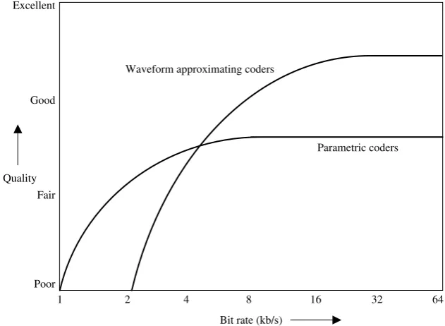
Major speech coders have been separated into two classes: waveform approx-imating coders and parametric coders. Kleijn [1] defines them as follows:
• Waveform approximating coders: Speech coders producing a
recon-structed signal which converges towards the original signal with decreasing quantization error.
• Parametric coders:Speech coders producing a reconstructed signal which
does not converge to the original signal with decreasing quantization error.
Typical performance curves for waveform approximating and parametric speech coders are shown in Figure 2.1. It is worth noting that, in the past, speech coders were grouped into three classes: waveform coders, vocoders and hybrid coders. Waveform coders included speech coders, such as PCM and ADPCM, and vocoders included very low bit-rate synthetic speech coders. Finally hybrid coders were those speech coders which used both of these methods, such as CELP, MBE etc. However currently all speech coders use some form of speech modelling whether their output converges to the
Poor Good
Fair Excellent
Quality
Bit rate (kb/s)
4 8 16 32 64
1 2
Waveform approximating coders
Parametric coders
Speech Coding Techniques 7
original (with increasing bit rate) or not. It is therefore more appropriate to group speech coders into the above two groups as the old waveform coding terminology is no longer applicable. If required we can associate the name hybrid coding with coding types that may use more than one speech coding principle, which is switched in and out according to the input speech signal characteristics. For example, a waveform approximating coder, such as CELP, may combine in an advantageous way with a harmonic coder, which uses a parametric coding method, to form such a hybrid coder.
2.2.1 Parametric Coders
Parametric coders model the speech signal using a set of model parameters. The extracted parameters at the encoder are quantized and transmitted to the decoder. The decoder synthesizes speech according to the specified model. The speech production model does not account for the quantization noise or try to preserve the waveform similarity between the synthesized and the original speech signals. The model parameter estimation may be an open loop process with no feedback from the quantization or the speech synthesis. These coders only preserve the features included in the speech production model, e.g. spectral envelope, pitch and energy contour, etc. The speech quality of parametric coders do not converge towards the transparent quality of the original speech with better quantization of model parameters, see Figure 2.1. This is due to limitations of the speech production model used. Furthermore, they do not preserve the waveform similarity and the measurement of signal to noise ratio (SNR) is meaningless, as often the SNR becomes negative when expressed in dB (as the input and output waveforms may not have phase alignment). The SNR has no correlation with the synthesized speech quality and the quality should be assessed subjectively (or perceptually).
Linear Prediction Based Vocoders
Harmonic Coders
Harmonic or sinusoidal coding represents the speech signal as a sum of sinu-soidal components. The model parameters, i.e. the amplitudes, frequencies and phases of sinusoids, are estimated at regular intervals from the speech spectrum. The frequency tracks are extracted from the peaks of the speech spectra, and the amplitudes and frequencies are interpolated in the synthesis process for smooth evolution [4]. The general sinusoidal model does not restrict the frequency tracks to be harmonics of the fundamental frequency. Increasing the parameter extraction rate converges the synthesized speech waveform towards the original, if the parameters are unquantized. However at low bit rates the phases are not transmitted and estimated at the decoder, and the frequency tracks are confined to be harmonics. Therefore point to point waveform similarity is not preserved.
2.2.2 Waveform-approximating Coders
Waveform coders minimize the error between the synthesized and the origi-nal speech waveforms. The early waveform coders such as companded Pulse Code Modulation (PCM) [5] and Adaptive Differential Pulse Code Mod-ulation (ADPCM) [6] transmit a quantized value for each speech sample. However ADPCM employs an adaptive pole zero predictor and quantizes the error signal, with an adaptive quantizer step size. ADPCM predictor coefficients and the quantizer step size are backward adaptive and updated at the sampling rate.
The recent waveform-approximating coders based on time domain analysis by synthesis such as Code Excited Linear Prediction (CELP) [7], explicitly make use of the vocal tract model and the long term prediction to model the correlations present in the speech signal. CELP coders buffer the speech signal and perform block based analysis and transmit the prediction filter coefficients along with an index for the excitation vector. They also employ perceptual weighting so that the quantization noise spectrum is masked by the signal level.
2.2.3 Hybrid Coding of Speech
Algorithm Objectives and Requirements 9
coding principles to encode different types of speech segments have been introduced [11, 12, 13].
A hybrid coder can switch between a set of predefined coding modes. Hence they are also referred to as multimode coders. A hybrid coder is an adaptive coder, which can change the coding technique or mode according to the source, selecting the best mode for the local character of the speech signal. Network or channel dependent mode decision [14] allows a coder to adapt to the network load or the channel error performance, by varying the modes and the bit rate, and changing the relative bit allocation of the source and channel coding [15].
In source dependent mode decision, the speech classification can be based on fixed or variable length frames. The number of bits allocated for frames of different modes can be the same or different. The overall bit rate of a hybrid coder can be fixed or variable. In fact variable rate coding can be seen as an extension of hybrid coding.
2.3 Algorithm Objectives and Requirements
The design of a particular algorithm is often dictated by the target application. Therefore, during the design of an algorithm the relative weighting of the influencing factors requires careful consideration in order to obtain a balanced compromise between the often conflicting objectives. Some of the factors which influence the choice of algorithm for the foreseeable network applications are listed below.
2.3.1 Quality and Capacity
2.3.2 Coding Delay
The coding delay of a speech transmission system is a factor closely related to the quality requirements. Coding delay may be algorithmic (the buffering of speech for analysis), computational (the time taken to process the stored speech samples) or due to transmission. Only the first two concern the speech coding subsystem, although very often the coding scheme is tailored such that transmission can be initiated even before the algorithm has completed pro-cessing all of the information in the analysis frame, e.g. in the pan-European digital mobile radio system (better known as GSM) [16] the encoder starts transmission of the spectral parameters as soon as they are available. Again, for PSTN applications, low delay is essential if the major problem of echo is to be minimized. For mobile system applications and satellite communication systems, echo cancellation is employed as substantial propagation delays already exist. However, in the case of the PSTN where there is very little delay, extra echo cancellers will be required if coders with long delays are introduced. The other problem of encoder/decoder delay is the purely sub-jective annoyance factor. Most low-rate algorithms introduce a substantial coding delay compared with the standard 64 kb/s PCM system. For instance, the GSM system’s initial upper limit was 65 ms for a back-to-back configura-tion, whereas for the 16 kb/s G.728 specification [17], it was a maximum of 5 ms with an objective of 2 ms.
2.3.3 Channel and Background Noise Robustness
For many applications, the speech source coding rate typically occupies only a fraction of the total channel capacity, the rest being used for forward error correction (FEC) and signalling. For mobile connections, which suffer greatly from both random and burst errors, a coding scheme’s built-in tolerance to channel errors is vital for an acceptable average overall performance, i.e. com-munication quality. By employing built-in robustness, less FEC can be used and higher source coding capacity is available to give better speech quality. This trade-off between speech quality and robustness is often a very difficult balance to obtain and is a requirement that necessitates consideration from the beginning of the speech coding algorithm design. For other applications employing less severe channels, e.g. fibre-optic links, the problems due to channel errors are reduced significantly and robustness can be ignored for higher clean channel speech quality. This is a major difference between the wireless mobile systems and those of the fixed link systems.
Algorithm Objectives and Requirements 11
regeneration by the coder is also an important requirement (unless adaptive noise cancellation is used before speech coding).
2.3.4 Complexity and Cost
As ever more sophisticated algorithms are devised, the computational com-plexity is increased. The advent of Digital Signal Processor (DSP) chips [18] and custom Application Specific Integrated Circuit (ASIC) chips has enabled the cost of processing power to be considerably lowered. However, complex-ity/power consumption, and hence cost, is still a major problem especially in applications where hardware portability is a prime factor. One technique for overcoming power consumption whilst also improving channel efficiency is digital speech interpolation (DSI) [16]. DSI exploits the fact that only around half of speech conversation is actually active speech thus, during inactive periods, the channel can be used for other purposes, including limiting the transmitter activity, hence saving power. An important subsystem of DSI is the voice activity detector (VAD) which must operate efficiently and reliably to ensure that real speech is not mistaken for silence and vice versa. Obvi-ously, a voice for silence mistake is tolerable, but the opposite can be very annoying.
2.3.5 Tandem Connection and Transcoding
As it is the end to end speech quality which is important to the end user, the ability of an algorithm to cope with tandeming with itself or with another coding system is important. Degradations introduced by tandeming are usually cumulative, and if an algorithm is heavily dependent on certain characteristics then severe degradations may result. This is a particularly urgent unresolved problem with current schemes which employ post-filtering in the output speech signal [17]. Transcoding into another format, usually PCM, also degrades the quality slightly and may introduce extra cost.
2.3.6 Voiceband Data Handling
Other solutions are often used. A very common one is to detect the voiceband data and use an interface which bypasses the speech encoder/decoder.
2.4 Standard Speech Coders
Standardization is essential in removing the compatibility and conforma-bility problems of implementations by various manufacturers. It allows for one manufacturer’s speech coding equipment to work with that of others. In the following, standard speech coders, mostly developed for specific communication systems, are listed and briefly reviewed.
2.4.1 ITU-T Speech Coding Standard
Traditionally the International Telecommunication Union Telecommunica-tion StandardizaTelecommunica-tion Sector (ITU-T, formerly CCITT) has standardized speech coding methods mainly for PSTN telephony with 3.4 kHz input speech band-width and 8 kHz sampling frequency, aiming to improve telecommunication network capacity by means of digital circuit multiplexing. Additionally, ITU-T has been conducting standardization for wideband speech coders to support 7 kHz input speech bandwidth with 16 kHz sampling frequency, mainly for ISDN applications.
Standard Speech Coders 13
Table 2.1 ITU-T narrowband speech coding standards
Bit rate Noise Delay
Speech coder (kb/s) VAD reduction (ms) Quality Year
G.711 (A/µ-Law PCM) 64 No No 0 Toll 1972
G.726 (ADPCM) 40/32/24/16 No No 0.25 Toll 1990
G.728 (LD-CELP) 16 No No 1.25 Toll 1992
G.729 (CSA-CELP) 8 Yes No 25 Toll 1996
G.723.1 6.3/5.3 Yes No 67.5 Toll/ 1995
(MP-MLQ/ACELP) Near-toll
G.4k (to be determined) 4 – Yes ∼55 Toll 2001
is a hybrid model of CELP and sinusoidal speech coding principles [27, 28]. A summary of the narrowband speech coding standards recommended by ITU-T is given in Table 2.1.
In addition to the narrowband standards, ITU-T has released two wideband speech coders, G.722 [29] and G.722.1 [30], targeting mainly multimedia communications with higher voice quality. G.722 [29] supports three bit rates, 64, 56, and 48 kb/s based on subband ADPCM (SB-ADPCM). It decomposes the input signals into low and high subbands using the quadrature mirror filters, and then quantizes the band-pass filtered signals using ADPCM with variable step sizes depending on the subband. G.722.1 [30] operates at the rates of 32 and 24 kb/s and is based on the transform coding technique. Currently, a new wideband speech coder operating at 13/16/20/24 kb/s is undergoing standardization.
2.4.2 European Digital Cellular Telephony Standards
With the advent of digital cellular telephony there have been many speech coding standardization activities by the European Telecommunications Stan-dards Institute (ETSI). The first release by ETSI was the GSM full rate (FR) speech coder operating at 13 kb/s [31]. Since then, ETSI has standardized 5.6 kb/s GSM half rate (HR) and 12.2 kb/s GSM enhanced full rate (EFR) speech coders [32, 33]. Following these, another ETSI standardization activity resulted in a new speech coder, called the adaptive multi-rate (AMR) coder [34], operating at eight bit rates from 12.2 to 4.75 kb/s (four rates for the full-rate and four for the half-rate channels). The AMR coder aims to provide enhanced speech quality based on optimal selection between the source and channel coding schemes (and rates). Under high radio interference, AMR is capable of allocating more bits for channel coding at the expense of reduced source coding rate and vice versa.
Table 2.2 ETSI speech coding standards for GSM mobile communications
Bit rate Noise Delay
Speech coder (kb/s) VAD reduction (ms) Quality Year
FR (RPE-LTP) 13 Yes No 40 Near-toll 1987
HR (VSELP) 5.6 Yes No 45 Near-toll 1994
EFR (ACELP) 12.2 Yes No 40 Toll 1998
AMR (ACELP) 12.2/10.2/7.95/ Yes No 40/45 Toll 1999
7.4/6.7/5.9/ ∼
Communi-5.15/4.75 cation
interference reduction as well as battery life time extension for mobile com-munications. Standard speech coders for European mobile communications are summarized in Table 2.2.
2.4.3 North American Digital Cellular Telephony Standards
In North America, the Telecommunication Industries Association (TIA) of the Electronic Industries Association (EIA) has been standardizing mobile communication based on Code Division Multiple Access (CDMA) and Time Division Multiple Access (TDMA) technologies used in the USA. TIA/EIA adopted Qualcomm CELP (QCELP) [39] for Interim Standard-96-A (IS-96-A), operating at variable bit rates between 8 kb/s and 0.8 kb/s controlled by a rate determination algorithm. Subsequently, TIA/EIA released IS-127 [40], the enhanced variable rate coder, which features a novel function for noise reduction as a preprocessor to the speech compression module. Under noisy background conditions, noise reduction provides a more comfortable speech quality by enhancing noisy speech signals. For personal communication systems, TIA/EIA released IS-733 [41], which operates at variable bit rates between 14.4 and 1.8 kb/s. For North American TDMA standards, TIA/EIA released IS-54 and IS-641-A for full rate and enhanced full rate speech coding, respectively [42, 43]. Standard speech coders for North American mobile communications are summarized in Table 2.3.
2.4.4 Secure Communication Telephony
Speech coding is a crucial part of a secure communication system, where voice intelligibility is a major concern in order to deliver the exact voice commands in an emergency.
Standard Speech Coders 15
Table 2.3 TIA/EIA speech coding standards for North American CDMA/TDMA mobile communications
Bit rate Noise Delay
Speech coder (kb/s) VAD reduction (ms) Quality Year IS-96-A (QCELP) 8.5/4/2/0.8 Yes No 45 Near-toll 1993 IS-127 (EVRC) 8.5/4/2/0.8 Yes Yes 45 Toll 1995 IS-733 (QCELP) 14.4/7.2/3.6/1.8 Yes No 45 Toll 1998
IS-54 (VSELP) 7.95 Yes No 45 Near-toll 1989
IS-641-A (ACELP) 7.4 Yes No 45 Toll 1996
Table 2.4 DoD speech coding standards
Bit rate Noise Delay
Speech coder (kb/s) VAD reduction (ms) Quality Year FS-1015 (LPC-10e) 2.4 No No 115 Intelligible 1984 FS-1016 (CELP) 4.8 No No 67.5 Communication 1991 DoD 2.4 (MELP) 2.4 No No 67.5 Communication 1996 STANAG (NATO) 2.4/1.2 No Yes >67.5 Communication 2001
2.4/1.2 (MELP)
on the mixed excitation linear prediction (MELP) vocoder [48] which is based on the sinusoidal speech coding model. The 2.4 kb/s DoD MELP speech coder gives better speech quality than the 4.8 kb/s FS-1016 coder at half the capacity. A modified and improved version of this coder, operating at dual rates of 2.4/1.2 kb/s and employing a noise preprocessor, has been selected as the new NATO standard. Parametric coders, such as MELP, have been widely used in secure communications due to their intelligible speech quality at very low bit rates. The DoD standard speech coders are summarized in Table 2.4.
2.4.5 Satellite Telephony
The international maritime satellite corporation (INMARSAT) has adopted two speech coders for satellite communications. INMARSAT has selected 4.15 kb/s improved multiband excitation (IMBE) [9] for INMARSAT M sys-tems and 3.6 kb/s advanced multiband excitation (AMBE) vocoders for INMARSAT Mini-M systems (see Table 2.5).
2.4.6 Selection of a Speech Coder
Table 2.5 INMARSAT speech coding standards
Bit rate Noise Delay
Speech coder (kb/s) VAD reduction (ms) Quality Year
IMBE 4.15 No No 120 Communication 1990
AMBE 3.6 No No – – –
Quality measurements based on SNR can be used to evaluate coders that preserve the waveform similarity, usually coders operating at bit rates above 16 kb/s. Low bit-rate parametric coders do not preserve the waveform simi-larity and SNR-based quality measures become meaningless. For parametric coders, perception-based subjective measures are more reliable. The Mean Opinion Score (MOS) [49] scale shown in Table 2.6 is a widely-used subjective quality measure.
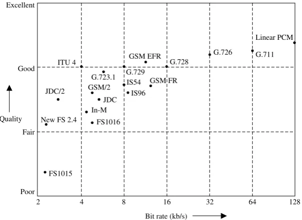
Table 2.7 compares some of the most well-known speech coding standards in terms of their bit rate, algorithmic delay and Mean Opinion Scores and Figure 2.2 illustrates the performance of those standards in terms of speech quality against bit rate [50, 51].
Linear PCM at 128 kb/s offers transparent speech quality and its A-law companded 8 bits/sample (64 kb/s) version (which provides the standard for the best (narrowband) quality) has a MOS score higher than 4, which is described as Toll quality. In order to find the MOS score for a given
FS1015
G.728
G.711 G.726
Linear PCM
G.729 G.723.1 ITU 4
GSM FR
FS1016
Poor
2 4 8 16 32 64 128
Good
Fair Excellent
Quality
Bit rate (kb/s) In-M
New FS 2.4
JDC
JDC/2 IS96
IS54 GSM/2
GSM EFR
Standard Speech Coders 17
Table 2.6 Mean Opinion Score (MOS) scale
Grade (MOS) Subjective opinion Quality 5 Excellent Imperceptible Transparent 4 Good Perceptible, but not annoying Toll
3 Fair Slightly annoying Communication
2 Poor Annoying Synthetic
1 Bad Very annoying Bad
Table 2.7 Comparison of telephone band speech coding standards
Standard Year Algorithm Bit rate (kb/s) MOS∗
Delay+
G.711 1972 Companded PCM 64 4.3 0.125
G.726 1991 VBR-ADPCM 16/24/32/40 toll 0.125
G.728 1994 LD-CELP 16 4 0.625
G.729 1995 CS-ACELP 8 4 15
G.723.1 1995 A/MP-MLQ CELP 5.3/6.3 toll 37.5
ITU 4 – – 4 toll 25
GSM FR 1989 RPE-LTP 13 3.7 20
GSM EFR 1995 ACELP 12.2 4 20
GSM/2 1994 VSELP 5.6 3.5 24.375
IS54 1989 VSELP 7.95 3.6 20
IS96 1993 Q-CELP 0.8/2/4/8.5 3.5 20
JDC 1990 VSELP 6.7 commun. 20
JDC/2 1993 PSI-CELP 3.45 commun. 40
Inmarsat-M 1990 IMBE 4.15 3.4 78.75
FS1015 1984 LPC-10 2.4 synthetic 112.5
FS1016 1991 CELP 4.8 3 37.5
New FS 2.4 1997 MELP 2.4 3 45.5
∗The MOS figures are obtained from formal subjective tests using varied test material (from the literature). These figures are therefore useful as a guide, but should not be taken as a definitive indication of codec performance.
+Delay is the total algorithmic delay, i.e. the frame length and look ahead, and is given in milliseconds.
give priority to some system parameters over others. In early speech coders, which aimed at reproducing the input speech waveform as output, objective measurement in the form of signal to quantization noise ratio was used. Since the bit rate of early speech coders was 16 kb/s or greater (i.e. they incurred only a small amount of quantization noise) and they did not involve complicated signal processing algorithms which could change the shape of the speech waveform, the SNR measures were reasonably accurate. However at lower bit rates where the noise (the objective difference between the original input and the synthetic output) increases, the use of signal to quantization noise ratio may be misleading. Hence there is a need for a better objective measurement which has a good correlation with the perceptual quality of the synthetic speech. The ITU standardized a number of these methods, the most recent of which is P.862 (or Perceptual Evaluation of Speech Quality). In this standard, various alignments and perceptual measures are used to match the objective results to fairly accurate subjective MOS scores.
2.5 Summary
Existing speech coders can be divided into three groups: parametric coders, waveform approximating coders, and hybrid coders. Parametric coders are not expected to reproduce the original waveform; they reproduce the per-ception of the original. Waveform approximating coders, on the other hand, are expected to replicate the input speech waveform as the bit rate increases. Hybrid coding is a combination of two or more coders of any type for the best subjective (and perhaps objective) performance at a given bit rate.
The design process of a speech coder involves several trade-offs between conflicting requirements. These requirements include the target bit rate, qual-ity, delay, complexqual-ity, channel error sensitivqual-ity, and sending of nonspeech signals. Various standardization bodies have been involved in speech coder standardization activities and as a result there have been many standard speech coders in the last decade. The bit rate of these coders ranges from 16 kb/s down to around 4 kb/s with target applications mainly in cellular mobile radio. The selection of a speech coder involves expensive testing under the expected typical operating conditions. The most popular testing method is subjective listening tests. However, as this is expensive and time-consuming, there has been some effort to produce simpler yet reliable objective measures. ITU P.862 is the latest effort in this direction.
Bibliography
Bibliography 19
[2] D. O’Shaughnessy (1987)Speech communication: human and machine. Addi-son Wesley
[3] I. Atkinson, S. Yeldener, and A. Kondoz (1997) ‘High quality split-band LPC vocoder operating at low bit rates’, inProc. of Int. Conf. on Acoust., Speech and Signal Processing, pp. 1559–62. May 1997. Munich
[4] R. J. McAulay and T. F. Quatieri (1986) ‘Speech analysis/synthesis based on a sinusoidal representation’, in IEEE Trans. on Acoust., Speech and Signal Processing, 34(4):744–54.
[5] ITU-T (1972)CCITT Recommendation G.711: Pulse Code Modulation (PCM) of Voice Frequencies. International Telecommunication Union.
[6] N. S. Jayant and P. Noll (1984)Digital Coding of Waveforms: Principles and applications to speech and video. New Jersey: Prentice-Hall
[7] B. S. Atal and M. R. Schroeder (1984) ‘Stochastic coding of speech at very low bit rates’, inProc. Int. Conf. Comm, pp. 1610–13. Amsterdam
[8] M. Schroeder and B. Atal (1985) ‘Code excited linear prediction (CELP): high quality speech at very low bit rates’, inProc. of Int. Conf. on Acoust., Speech and Signal Processing, pp. 937–40. Tampa, FL
[9] DVSI (1991) INMARSAT-M Voice Codec, Version 1.7. September 1991. Digital Voice Systems Inc.
[10] J. C. Hardwick and J. S. Lim (1991) ‘The application of the IMBE speech coder to mobile communications’, inProc. of Int. Conf. on Acoust., Speech and Signal Processing, pp. 249–52.
[11] W. B. Kleijn (1993) ‘Encoding speech using prototype waveforms’, in IEEE Trans. Speech and Audio Processing, 1:386–99.
[12] E. Shlomot, V. Cuperman, and A. Gersho (1998) ‘Combined harmonic and waveform coding of speech at low bit rates’, inProc. of Int. Conf. on Acoust., Speech and Signal Processing.
[13] J. Stachurski and A. McCree (2000) ‘Combining parametric and waveform-matching coders for low bit-rate speech coding’, inX European Signal Processing Conf.
[14] T. Kawashima, V. Sharama, and A. Gersho (1994) ‘Network control of speech bit rate for enhanced cellular CDMA performance’, inProc. IEE Int. Conf. on Commun., 3:1276.
[15] P. Ho, E. Yuen, and V. Cuperman (1994) ‘Variable rate speech and channel coding for mobile communications’, inProc. of Vehicular Technology Conf. [16] J. E. Natvig, S. Hansen, and J. de Brito (1989) ‘Speech processing in the pan-European digital mobile radio system (GSM): System overview’, in Proc. of Globecom, Section 29B.
[18] E. Lee (1988) ‘Programmable DSP architectures’, inIEEE ASSP Magazine, October 1988 and January 1989.
[19] ITU-T (1988)Pulse code modulation (PCM) of voice frequencies, ITU-T Rec. G.711.
[20] ITU-T (1990) 40, 32, 24, 16 kbit/s adaptive differential pulse code modulation (ADPCM), ITU-T Rec. G.726.
[21] ITU-T (1996) Dual rate speech coder for multimedia communications trans-mitting at 5.3 and 6.3 kbit/s, ITU-T Rec. G.723.1.
[22] ITU-T (1992)Coding of speech at 16 kbit/s using low-delay code excited linear prediction, ITU-T Rec. G.728.
[23] ITU-T (1996)Coding of speech at 8 kbit/s using conjugate-structure algebraic-code-excited linear prediction (CS-ACELP), ITU-T Rec. G.729.
[24] ITU-T (1996)A silence compression scheme for G.729 optimised for terminals conforming to ITU-T V.70, ITU-T Rec. G.729 Annex B.
[25] ITU-T (1996)Dual rate speech coder for multimedia communications transmit-ting at 5.3 and 6.3 kbit/s. Annex A: Silence compression scheme, ITU-T Rec. G.723.1 Annex A.
[26] O. Hersent, D. Gurle, and J. Petit (2000)IP Telephony: Packet-based multi-media communications systems. Addison Wesley
[27] J. Thyssen, Y. Gao, A. Benyassine, E. Shylomot, H. -Y. Su, K. Mano, Y. Hiwasaki, H. Ehara, K. Yasunaga, C. Lamblin, B. Kovest, J. Stegmann, and H. -G. Kang (2001) ‘A candidate for the ITU-T 4 kbit/s speech coding standard’, in Proc. of Int. Conf. on Acoust., Speech and Signal Processing. May 2001. Salt Lake City, UT
[28] J. Stachurski and A. McCree (2000) ‘A 4 kb/s hybrid MELP/CELP coder with alignment phase encoding and zero phase equalization’, inProc. of Int. Conf. on Acoust., Speech and Signal Processing, pp. 1379–82. May 2000. Istanbul
[29] ITU-T (1988)7 khz audio-coding within 64 kbit/s, ITU-T Rec. G.722.
[30] ITU-T (1999) Coding at 24 and 32 kbit/s for hands-free operation in systems with low frame loss, ITU-T Rec. G.722.1
[31] ETSI (1994)Digital cellular telecommunications system (phase 2+); Full rate
speech transcoding, GSM 06.10 (ETS 300 580-2).
[32] ETSI (1997)Digital cellular telecommunications system (phase 2+); Half rate
speech; Half rate speech transcoding, GSM 06.20 v5.1.0 (draft ETSI ETS 300 969).
[33] ETSI (1998) Digital cellular telecommunications system (phase 2); Enhanced full rate (EFR) speech transcoding, GSM 06.60 v4.1.0 (ETS 301 245), June. [34] ETSI (1998)Digital cellular telecommunications system (phase 2+); Adaptive
Bibliography 21
[35] ETSI (1998) Digital cellular telecommunications system (phase 2+); Voice
activity detector (VAD) for full rate speech traffic channels, GSM 06.32 (ETSI EN 300 965 v7.0.1).
[36] ETSI (1999) Digital cellular telecommunications system (phase 2+); Voice
activity detector (VAD) for full rate speech traffic channels, GSM 06.42 (draft ETSI EN 300 973 v8.0.0).
[37] ETSI (1997)Digital cellular telecommunications system; Voice activity detector (VAD) for enhanced full rate (EFR) speech traffic channels, GSM 06.82 (ETS 300 730), March.
[38] ETSI (1998) Digital cellular telecommunications system (phase 2+); Voice
activity detector (VAD) for adaptive multi-rate (AMR) speech traffic channels, GSM 06.94 v7.1.1 (ETSI EN 301 708).
[39] P. DeJaco, W. Gardner, and C. Lee (1993) ‘QCELP: The North American CDMA digital cellular variable rate speech coding standard’, in IEEE Workshop on Speech Coding for Telecom, pp. 5–6.
[40] TIA/EIA (1997) Enhanced variable rate codec, speech service option 3 for wideband spread spectrum digital systems, IS-127.
[41] TIA/EIA (1998) High rate speech service option 17 for wideband spread spectrum communication systems, IS-733.
[42] I. A. Gerson and M. A. Jasiuk (1990) ‘Vector sum excited linear prediction (VSELP) speech coding at 8 kb/s’, inProc. of Int. Conf. on Acoust., Speech and Signal Processing, pp. 461–4. April 1990. Albuquerque, NM, USA [43] T. Honkanen, J. Vainio, K. Jarvinen, and P. Haavisto (1997) ‘Enhanced full
rate speech coder for IS-136 digital cellular system’, inProc. of Int. Conf. on Acoust., Speech and Signal Processing, pp. 731–4. May 1997. Munich [44] T. E. Tremain (1982) ‘The government standard linear predictive coding
algorithm: LPC-10’, inSpeech Technology, 1:40–9.
[45] J. P. Campbell Jr and T. E. Tremain (1986) ‘Voiced/unvoiced classification of speech with applications to the US government LPC-10e algorithm’, inProc. of Int. Conf. on Acoust., Speech and Signal Processing, pp. 473–6. [46] J. P. Campbell, V. C. Welch, and T. E. Tremain (1991) ‘The DoD 4.8 kbps
standard (proposed Federal Standard 1016)’, inAdvances in Speech Coding by B. Atal, V. Cuperman, and A. Gersho (Eds), pp. 121–33. Dordrecht, Holland: Kluwer Academic
[47] FIPS (1997) Analog to digital conversion of voice by 2,400 bit/second mixed excitation linear prediction (MELP), Draft. Federal Information Processing Standards
[48] A. V. McCree and T. P. Barnwell (1995) ‘A mixed excitation LPC vocoder model for low bit rate speech coding’, in IEEE Trans. Speech and Audio Processing, 3(4):242–50.
[50] R. V. Cox (1995) ‘Speech coding standards’, inSpeech coding and synthesis by W. B. Kleijn and K. K. Paliwal (Eds), pp. 49–78. Amsterdam: Elsevier Science
3
Sampling and Quantization
3.1 Introduction
In digital communication systems, signal processing tools require the input source to be digitized before being processed through various stages of the network. The digitization process consists of two main stages: sampling the signal and converting the sampled amplitudes into binary (digital) code-words. The difference between the original analogue amplitudes and the digitized ones depend on the number of bits used in the conversion. A 16 bit analogue to digital converter is usually used to sample and digitize the input analogue speech signal. Having digitized the input speech, the speech coding algorithms are used to compress the resultant bit rate where various quan-tizers are used. In this chapter, after a brief review of the sampling process, quantizers which are used in speech coders are discussed.
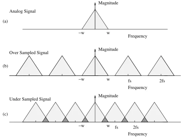
3.2 Sampling
As stated above, the digital conversion process can be split into sampling, which discretizes the continuous time, and quantization, which reduces the infinite range of the sampled amplitudes to a finite set of possibilities. The sampled waveform can be represented by,
s(n)=sa(nT) − ∞<n<∞ (3.1)
wheresais the analogue waveform,nis the integer sample number andTis the
sampling time (the time difference between any two adjacent samples, which is determined by the bandwidth or the highest frequency in the input signal).
The sampling theorem states that if a signalsa(t)has a band-limited Fourier
transformSa(jω)given by,
Sa(jω)=
∞
−∞
sa(t)e−jωtdt (3.2)
such that Sa(jω) = 0 for|ω| ≥ 2πW then the analogue signal can be
recon-structed from its sampled version if T ≤ 1/2W. W is called the Nyquist frequency.
The effect of sampling is shown in Figure 3.1. As can be seen from Figures 3.1b and 3.1c, the band-limited Fourier transform of the analogue signal which is shown in Figure 3.1a is duplicated at every multiple of the sampling frequency.
This is because the Fourier transform of the sampled signal is evaluated at multiples of the sampling frequency which forms the relationship,
S(ejωT)= 1 T
∞
n=−∞
Sa(jω+j2πn/T) (3.3)
This can also be interpreted by looking into the time domain sampling process where the input signal is regularly (at every sampling interval) multiplied
Frequency Frequency Frequency
2fs fs
2fs fs
w w w −w
−w
−w (c)
(b) (a)
Under Sampled Signal Over Sampled Signal Analog Signal
Magnitude
Magnitude Magnitude
Sampling 25
with a delta function. When converted to the frequency domain, the multi-plication becomes convolution and the message spectrum is reproduced at multiples of the sampling frequency.
We can clearly see that if the sampling frequency is less than twice the Nyquist frequency, the spectra of two adjacent multiples of the sampling frequencies will overlap. For example, if T1 = fs < 2W the analogue signal
image centred at 2π/T overlaps into the base band image. The distortion caused by high frequencies overlapping low frequencies is calledaliasing. In order to avoid aliasing distortion, either the input analogue signal has to be band-limited to a maximum of half the sampling frequency or the sampling frequency has to be increased to at least twice the highest frequency in the analogue signal.
Given the condition 1/T > 2W, the Fourier transform of the sampled sequence is proportional to the Fourier transform of the analogue signal in the base band as follows:
S(ejωT)= 1
TSa(jω) |ω|< π
T (3.4)
Using the above relationship, the original analogue signal can be obtained from the sampled sequence using interpolation given by [1],
sa(t)= ∞
n=−∞
sa(nT)sin[π(t
−nT)/T]
π(t−nT)/T (3.5)
which can be written as,
sa(t)= ∞
n=−∞
sa(nT)sinc(φ) (3.6)
whereφ =π(t−nT)/T.
3.3 Scalar Quantization
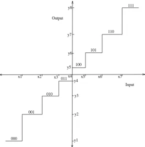
Quantization converts a continuous-amplitude signal (usually 16 bit, rep-resented by the digitization process) to a discrete-amplitude signal that is different from the continuous-amplitude signal by the quantization error or noise. When each of a set of discrete values is quantized separately the process is known as scalar quantization. The input–output characteristics of a uniform scalar quantizer are shown in Figure 3.2.
Each sampled value of the input analogue signal, which has an infinite range (16 bit digitized), is compared against a finite set of amplitude values and the closest value from the finite set is chosen to represent the amplitude. The distance between the finite set of amplitude levels is called the quantizer step size and is usually represented by . Each discrete amplitude level xi
is represented by a codewordc(n)for transmission purposes. The codeword
c(n) indicates to the de-quantizer, which is usually at the receiver, which discrete amplitude is to be used.
Assuming all of the discrete amplitude values in the quantizer are repre-sented by the same number of bits B and the sampling frequency is fs, the
Input Output
x4 x3 x2
x1 x5 x6 x7
y8
y7
y6
y5
y4
y3
y2
y1 101
000
001 010
100
110 111
011
Scalar Quantization 27
channel transmission bit rate is given by,
Tc=Bfs bits/second (3.7)
Given a fixed sampling frequency, the only way to reduce the channel bit rateTc is by reducing the length of the codewordc(n). However, a reduced
lengthc(n)means a smaller set of discrete amplitudes separated by larger
and, hence, larger differences between the analogue and discrete amplitudes after quantization, which reduces the quality of reconstructed signal. In order to reduce the bit rate while maintaining good speech quality, various types of scalar quantizer have been designed and used in practice. The main aim of a specific quantizer is to match the input signal characteristics both in terms of its dynamic range and probability density function.
3.3.1 Quantization Error
When estimating the quantization error, we cannot assume thati =i+nif
the quantizer is not uniform [2]. Therefore, the signal lying in theithinterval,
xi− i
2 ≤s(n) <xi+
i
2 (3.8)
is represented by the quantized amplitudexiand the difference between the
input and quantized values is a function of i. The instantaneous squared error, for the signal lying in theith interval is(s(n)−xi)2. The mean squared
error of the signal can then be written by including the likelihood of the signal being in theithinterval as,
E2i =
xi+i
2
xi−2i
(x−xi)2p(x)dx (3.9)
wheres(n)has been replaced byxfor ease of notation andp(x)represents the probability density function ofx. Assuming the step sizeiis small, enabling very fine quantization, we can assume that p(x) is flat within the interval
xi−2 toxi+2. Representing the flat region ofp(x)by its value at the centre, p(xi), the above equation can be written as,
E2i =p(xi)
The probability of the signal falling in theithinterval is,
Ŵi=
xi+i
2
xi−2i
The above is true only if the quantization levels are very small and, hence,
p(x)in each interval can be assumed to be uniform. Substituting (3.11) into (3.10) forp(xi)we get,
E2i = 2 i
12Ŵi (3.12)
The total mean squared error is therefore given by,
E2= 1
12
N
i=1
Ŵi2i (3.13)
whereNis the total number of levels in the quantizer. In the case of a uniform quantizer where each step size is the same, , the total mean squared error becomes,
E2 = 2
12
N
i=1
Ŵi = 2
12 (3.14)
where we assume that the signal amplitude is always in the quantizer range and, hence,N
i=1Ŵi =1.
3.3.2 Uniform Quantizer
The input–output characteristics of a uniform quantizer are shown in Figure 3.2. As can be seen from its input–output characteristics, all of the quantizer intervals (steps) are the same width. A uniform quantizer can be defined by two parameters: the number of quantizer levels and the quantizer step size . The number of levels is generally chosen to be of the form 2B, to make the most efficient use ofB bit binary codewords.andB must be chosen together to cover the range of input samples. Assuming |x| ≤ Xmax
and that the probability density function ofxis symmetrical, then,
2Xmax=2B (3.15)
From the above equation it is easily seen that once the number of bits to be used,B, is known, then the step size,, can be calculated by,
= 2Xmax
2B (3.16)
The quantization erroreq(n)is bounded by,
−
2 ≤eq(n)≤
Scalar Quantization 29
In a uniform quantizer, the only way to reduce the quantization error is by increasing the number of bits. When a uniform quantizer is used, it is assumed that the input signal has a uniform probability density function varying between±Xmaxwith a constant height of 2X1max. From this, the power
of the input signal can be written as,
Px= Xmax
−Xmax
x2p(x)dx= X 2 max
3 (3.18)
Using the result of (3.14), the signal to noise ratio can be written as,
SNR= Px Pn
= X
2 max/3
2/12 (3.19)
Substituting (3.16) forwe get,
SNR= Px Pn
=22B (3.20)
Taking the log,
SNR(dB)=10 log10(22B)=20Blog10(2)=6.02B dB (3.21)
The above result is useful both in determining the number of bits needed in the quantizer for certain signal to quantization noise ratio and in estimating the performance of a uniform quantizer for a given bit rate.
3.3.3 Optimum Quantizer
Input Output
x4 x5
y5
y4
x1 x2 x3 x6 x7
y3
y2 y8
y7
y6
y1 100
110
111
101
001
000
010 011
Figure 3.3 The input–output characteristics of a nonuniform quantizer
compressor,C(x), compresses the input samples depending on their statistical properties. In other words, the less likely higher sample values are compressed more than the more likely low amplitude samples. The compressed samples are then quantized using a uniform quantizer. The effect of compression is reversed at the receiver by applying the inverse C−1(x) expansion to the de-quantized samples. The compression and expansion processes do not introduce any signal distortions.
It is quite important to select the best compression–expansion combination for a given input signal probability density function. Panter and Dite [3] used analysis based on the assumption that the quantization is sufficiently fine and that the amplitude probability density function of the input samples is constant within the quantization intervals. Their results show significant improvement in the signal to noise ratio over uniform quantization if the input samples have apeakto root mean squared (rms) ratio greater than 4.
Scalar Quantization 31
Table 3.1 Max quantizer input and output levels for 1, 2, 3, 4, and 5 bit quantizers
Max quantizer thresholds
1 bit 2 bit 3 bit 4 bit 5 bit
i/p o/p i/p o/p i/p o/p i/p o/p i/p o/p
0.0000 0.7980 0.0000 0.4528 0.0000 0.2451 0.0000 0.1284 0.0000 0.0659 0.9816 1.5100 0.5006 0.7560 0.2582 0.3881 0.1320 0.1981 1.0500 1.3440 0.5224 0.6568 0.2648 0.3314 1.7480 2.1520 0.7996 0.9424 0.3991 0.4668 1.0990 1.2560 0.5359 0.6050 1.4370 1.6180 0.6761 0.7473 1.8440 2.0690 0.8210 0.8947 2.4010 2.7330 0.9718 1.0490 1.1300 1.2120 1.2990 1.3870 1.4820 1.5770 1.6820 1.7880 1.9080 2.0290 2.1740 2.3190 2.5050 2.6920 2.9770 3.2630
variance,σx2, of the input signal but made no assumption of fine quantization. The quantizer input–output threshold values for 1–5 bit Max quantizers are tabulated in Table 3.1 [4]. The quantizers in Table 3.1 are for a unit variance signal with a normal probability density function. Each quantizer has the same threshold values in the corresponding negative side of the quantizer.
Nonuniform quantization is advantageous in speech coding, both in coarse and fine quantization cases, for two reasons. Firstly, a nonuniform quantizer matches the speech probability density function better and hence produces higher signal to noise ratio than a uniform quantizer. Secondly, lower ampli-tudes, which contribute more to the intelligibility of speech, are quantized more accurately in a nonuniform quantizer.