MASSIVE-SCALE TREE MODELLING FROM TLS DATA
P. Raumonena,∗, E. Casellab
, K. Caldersc, S. Murphyd, M. ˚Akerbloma, M. Kaasalainena
aTampere University of Technology, Tampere, Finland- (pasi.raumonen, mikko.kaasalainen, markku.akerblom)@tut.fi b
Forest Research, Farnham, UK- [email protected] cWageningen University, Wageningen, Netherlands- [email protected] d
Melbourne School of Land and Environment, University of Melbourne, Australia- [email protected]
KEY WORDS:Quantitative structure models, automatic tree extraction, biomass, forest plot, ground truth, oak, eucalyptus, LiDAR
ABSTRACT:
This paper presents a method for reconstructing automatically the quantitative structure model of every tree in a forest plot from terrestrial laser scanner data. A new feature is the automatic extraction of individual trees from the point cloud. The method is tested with a 30-m diameter English oak plot and a 80-m diameter Australian eucalyptus plot. For the oak plot the total biomass was overestimated by about 17 %, when compared to allometry (N = 15), and the modelling time was about 100 min with a laptop. For the eucalyptus plot the total biomass was overestimated by about 8.5 %, when compared to a destructive reference (N = 27), and the modelling time was about 160 min. The method provides accurate and fast tree modelling abilities for, e.g., biomass estimation and ground truth data for airborne measurements at a massive ground scale.
1. INTRODUCTION
The measurement of above-ground forest biomass is important for ecology, carbon storage estimation, forest research, etc. Cur-rently airborne and satellite-based remote sensing is needed to es-timate the biomass of large forest areas. These measurements re-quire calibration based on good quality reference or ground truth data from test sites. Furthermore, it should be possible to measure the reference data quickly, cheaply, and nondestructively. The traditional way is to use allometry, but this can be problematic as errors can be in some cases over 30% (Calders et al. 2015).
With terrestrial laser scanning (TLS) and computational meth-ods it is now possible to automatically reconstruct accurate and precise 3D models of the tree structure of the scanned trees in minutes (Raumonen et al. 2013, Calders et al. 2015). We call these modelsquantitative structure modelsor QSMs. They rep-resent the trees as hierarchical collections of cylinders or other building blocks which provide the volume and diameter of branch segments needed to estimate the biomass. From QSMs it is thus possible to accurately and non-destructively estimate the volume, branching structure and branch size distribution and also detect growth and changes (Kaasalainen et al. 2014). Notice that the building blocks approach makes the models discontinuous, but this does not affect the modelled structural parameters. Overall, the circular cylinder is the best choice for a block type ( ˚Akerblom et al. 2014).
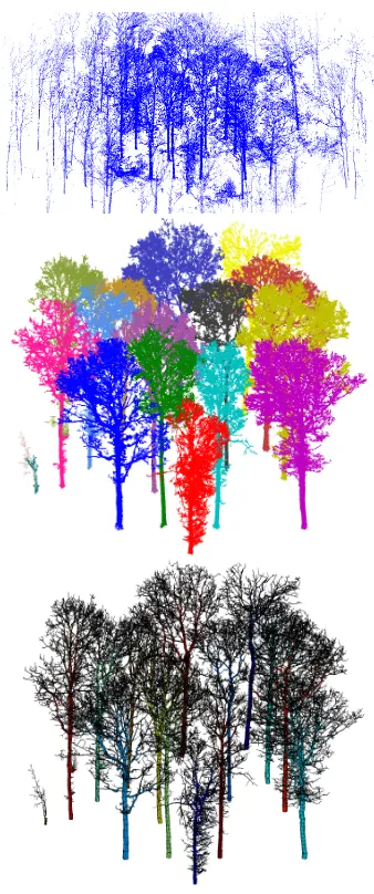
Our method and most other automatic reconstruction methods so far have been working only for scans with single trees, i.e., a manual extraction of the trees from the scans was required. In this paper we presentautomatic reconstruction for plot level. In other words, we use the “raw data” of the scans, which contain all the trees in the plot and measurements from ground and understory. The scans are only registered into a common coordinate system and then all the individual trees are automatically extracted and the QSMs are reconstructed. Fig. 1 shows an example of tree extraction and QSM reconstruction for a plot with a 15-m radius (modelling time about 100 min with a laptop).
∗Corresponding author
Plot-level tree modelling is thus very fast and also makes the tree extraction faster and more reliable. Extracting individual trees manually from large point clouds is time consuming (a couple of hours for one oak tree), and if the branches of neighbouring trees overlap, the manual separation is not easy or reliable. There are of course challenges also in automatic tree extraction, and it is probably impossible to make an algorithm that could always extract trees without any errors, especially for dense forests. We demonstrate and test our method with an English oak leaf-off plot and an Australian leaf-on eucalyptus plot.
Very large point clouds may require algorithms optimising mem-ory usage and computation times. For example, parallel com-puting can be used to simultaneously reconstruct the QSMs for each tree. Our demonstration uses 15-m and 40-m radius plots, but the method can be easily applied to much larger areas while the memory and computation time increase linearly with the plot area. Thus it is possible to scan and automatically model, e.g., multi-hectare-size plots.
There are a number of other methods for reconstructing single trees from TLS-data, e.g. (Dassot et al 2012, Hackenberg et al. 2014), but these require (semi-)manual tree extraction. There are automatic methods for some inventory data, such as dbh, volume and height, from TLS data, e.g. (Hopkins et al. 2004, Maas et al. 2008). Eysn et al. (2013) presented a fast but manual method for separating the stems and biggest branches from plot-level data.
The paper is organised as follows. In section 2 we introduce the data, present the details of the extraction and reconstruction method and a sensitivity analysis. In Section 3 we present the results, and sections 4 and 5 contain discussion and conclusions.
2. MATERIALS AND METHODS
In this section we first present the data used for the examples, then we give an outline of the reconstruction method, present the de-tails of the tree extraction and reconstruction methods, and finally go over some sensitivity analysis.
2.1 Measurements
We have measurements from two contrasting forest plots col-lected with different scanners and setups. The first plot is an 80-year-old oak plantation in South-Eastern England (51.1533◦ N; 0.8512◦W; 82 m asl). The plantation covers a total ground area of about 85 ha, managed as a commercial forest of mixed species dominated at 75% byQuercus robur L. The stocking den-sity was 405 trees per ha in 2011, with a mean height of 23+/-2 m. The understory was dominated by hazel (Corylus avellana L.) and hawthorn (Crataegus monogyna Jacq.) bushes. A 30 x 30 m experimental area was selected and the understory removed before data acquisition. We have a reference for dry mass (DM, in kilograms) given by an empirical relation computed from the diameter at breast height (DBH, in meters):
DM = 14720DBH2.8682. (1)
The wood density used for converting the modelled volume to dry mass is 507+/-40kg/m3
. Five scan locations was used for this study, one in the centre and the others near the boundary of the plot. They were recorded in April 2012 (leaf-off, no precipitation, wind speed averaged over the acquisition period was 0.7+/- 0.5 m/s).
The other plot is part of native Eucalyptus open forest (dry sclero-phyll Box-Ironbark forest) in Victoria, Australia (36◦45′36.49”S;
145◦0′59.58”E). The plot, called RUSH06, has a 40-m radius and it was established in Rushworth forest and partially harvested in May 2012 to acquire accurate estimates of biomass. The main tree species in the plot were Eucalyptus leucoxylon, E. micro-carpaandE. tricarpa. Five scan locations, with one in the centre and four 40 m from the centre, were used (Calders et al 2015).
The oak plot was scanned with the field portable (15 kg), phase-shift range finder, single return, HDS-6100 (Leica Geosystems Ltd., Heerbrugg) with a rotating mirror system that can cover a 310◦in zenith by 360◦in azimuth field of view. The beam wave-length is within the red band (650-690 nm) with a 0.003 m spot size at exit and a divergence angle of 0.013◦. The angular sam-pling resolution was 0.036◦in both directions. The maximum detection range is about 80 m. The scanner was mounted on a tri-pod with the laser source located at about 1.3 m above the ground. For each location, one full scan (310◦x 360◦) was recorded. The final co-registered point cloud has about 124 million points.
The eucalyptus plot was scanned with a RIEGL VZ-400 (RIEGL Laser Measurement Systems GmbH). The beam divergence is 0.02◦and the instrument operates in the infrared band (1550 nm) with a detection range up to 350 m. The angular sampling reso-lution was 0.06◦in both directions. The scanner allows fast data acquisition and records multiple return LiDAR data (up to four re-turns per emitted pulse). The advantage of multiple rere-turns over single returns is the improved sampling at greater canopy heights (Calders et al. 2014). Because RIEGL VZ-400 has a zenith range of 30 to 130 degrees, an additional scan was acquired at each scan location with the instrument tilted at 90 degrees to sample a full hemisphere. The final co-registered point cloud has about 71 million points.
For both plots, reflecting targets (six 15 cm black & white tilt & turn targets for the oak plot) were distributed throughout the plot area and were used to co-register the five scan locations using the Cyclone (Leica Geosystems, version 9) and the RiSCAN PRO (provided by RIEGL). The error in the co-registration of point clouds was 0.125+/-0.075 cm for the Oak plot (individual scans ranging from 0-3 mm), and 1.29 cm (ranging from 0.62 cm to 2.26 cm) for the eucalyptus plot.
2.2 Outline of the Method
The method is based on morphological rules, a cover-set approach, and geometric primitives. By morphological rules we mean that the reconstruction steps follow the tree topology and the major shape characteristics. The cover-set approach means a technical aspect of how point clouds are filtered and segmented, first into trees and then into branches, by concentrating on the smallest meaningful parts or units (surface patches) on the tree surface. The surfaces and structures of the trees are reconstructed with suitable geometric primitives; in this paper with cylinders.
The first major but optional step in the method isfiltering. We fil-ter out noise, remove some ground and understory points, include only the points within a given plot size, and make regions of very high point density sparser (to save memory).
into individual trees following botanical rules: first determine the stems one-by-one, then the 1st-order branches one-by-one, then the 2nd-order branches, etc. In cases where the trees are sepa-rated from each other by large enough distances between their closest branches, the segmentation process extracts the individ-ual trees reliably. When there are some contacts between the branches from different trees (or the gaps between the trees are small), we can still expect a reasonably good separation of trees. At this point further heuristic correction steps can be included.
The third and final major step is thereconstruction of QSMsfor each tree individually. The QSM reconstruction has been vali-dated earlier (Calders et al. 2015). Again the point cloud is cov-ered with patches, this time with smaller and variable size that de-creases as the branches get smaller. The variable size is based on the information from the first segmentation used for tree extrac-tion. The patches are again segmented into stems and branches as earlier, and finally each segment is partitioned into smaller re-gions for cylinder fitting.
We have made a short video demonstrating the method ( ˚Akerblom 2014).
2.3 Technical tools
Before going into the details of the major steps in the method, we discuss briefly some technical but necessary tools we need.
2.3.1 Cubical partition To handle a large number of points effectively without requiring huge amount of memory and to avoid pointless computations, it is useful to partition the point clouds into smaller cubical regions. The coordinatesQof the cubical region where each point belongs are computed from 1) the coor-dinatesPof the points; 2) the “lowest corner”CLof the cubical partition space (usually the minima of the x,y,z-coordinates); and 3) the edge lengtheof the cubes:Q=f loor[(P−CL)/e] + 1. Heref loordenotes rounding to the nearest smaller integer, and the three components [QX, QY, QZ]of Qare between 1 and the number of cubes (NX, NY, NZ) in the sides of this cubi-cal space. One way to quickly determine the points in the same cubes is to use the lexicographical coordinateL ofQ: L =
QX+ (QY −1)NX+ (QZ−1)NXNY. Points are sorted into increasingL-values and the consecutive points with the sameL -values are selected to form each cube.
For a fast way of finding neighbouring cubes, thee-cubes should be recorded also as a 3D-cell array, where the coordinatesQgive also the cell coordinates. However, with smalle-values compared to the size of the space, the number of cubes can be so large that there is not enough memory to store all the cells. Fortunately, because the points are from the surfaces of trees, the whole space is often quite sparsely filled. Thus it is possible to partition the space first into much larger cubes with an edge length E, e.g. 1-10 m, in which case the number ofE-cubes is only a small fraction compared toe-cubes and still most of theE-cubes will be empty. Then we select only the nonemptyE-cubes and ex-pand them to include one layer of neighbouringe-cubes from the neighbouringE-cubes. The point cloud is thus partitioned into an array of nonemptyE-cubes, which are further partitioned into 3D-cell arrays of empty and nonemptye-cubes.
2.3.2 Cover Sets The cover sets of a point cloud sampling the surfaces of trees and other objects are small subsets correspond-ing to surface patches on the surfaces of the objects. The idea is to partition the surfaces into small sets that 1) are in some sense the smallest meaningful subsets corresponding to the details of the branching structure, and 2) conform to the local shape of the surface, i.e., correspond to connected surface patches. This is in
contrast to voxel approaches, where the boundaries of the voxels are completely arbitrary with respect to the shape and the exact location of the details of the surface.
The process has two basic steps and the sets are randomly but about evenly covered along the surface of the tree with some re-strictions. First we generater-balls such that 1) the centres of the balls have at least a distancedbetween them such thatd ≤ r
holds, 2) each point is at most the distancedaway from its clos-est centre, and 3) an acceptable ball has at leastnpoints. These balls can now overlap, which is exploited later. Second, each ball defines acover setas those points of the ball that are closest to its centre. The cover sets thus do not overlap but form a partition of the points. Finally we define neighbour relations for the cover sets: two cover sets are neighbours if theirr-balls intersect. This neighbour relation can be used as a convenient tool for expanding or moving along the surface or for determining connected com-ponents (Raumonen et al. 2013).
The generation can be realised using a cubical partition of points intor-cubes. To determine ther-ball for the pointp, we take the
r-cube ofpand its 26 neighbouring cubes to restrict the search to nearby points. More details can be found in Raumonen et al. 2013. To save memory with very large point clouds, it is possible to carry out a cover generation without saving the partition: when a largeE-cube containing itsr-cubes is defined, use it directly for the cover generation of that cubical region and then proceed to define the nextE-cube and its cover generation.
2.4 Filtering
The first major step in the method is the filtering of the points that are not detections of a tree surface. Another aim here is to reduce the size of the point cloud so that the memory and computation time requirements can be reduced. First we remove points from ground and small understory as well as points that are too far away from the plot centre. Second, especially for high resolution scans the point density near the scanner may be unnecessarily high, and to reduce the number of points, we randomly remove some of these points. Finally, we try to remove noise, i.e., points that are not clear samples of any surface but are generated by the scanning process itself, e.g., by an error on range estimates due to the footprint of the laser hitting a limb.
First the point cloud is restricted by removing all the points whose horizontal distance from the plot’s centre is 20 m over the plot’s radius. Next the points are partitioned into horizontally defined rectangular regions and the bottom (ground and understory) is removed: The side length of these rectangles is set to, e.g., 0.5 m and the minimum and maximum z-valuesZLandZHfor each rectangle are determined. IfZH> ZL+ 0.5m holds, we remove the points for whichZ < ZL+ 0.25m holds.
Next we use the cubical partition of the already filtered point cloud to modify regions with too small or too high point den-sities: remove the points in cubes that have fewer points than some given threshold, and thin out cubes with more points than some threshold by randomly selecting a smaller sample. Here the cubes are considered separately without considering their neigh-bours. For the eucalyptus plot we used 10 cm cubes with 7 points as the minimum threshold and 150 points as the maximum one. The oak plot has a higher resolution: we used 10 cm cubes with 10 points as the minimum and 150 points for the maximum.
r-balls withralso as the minimum distance between the centres and the maximum distance from any point to its closest centre. For both plots we usedr = 6cm. Then all the points that be-long to a ball with more points than some given threshold (5 was used for both plots) are kept and others removed. Notice that a point may belong to multiple overlapping balls and it is assigned to the ball containing the most points. After this a new cover of the filtered point cloud using new set of parameters (r,d) is gen-erated. The connected components of this cover are determined and all components with less sets than some given threshold are removed. For both plots we usedr = 6cm,d= 5cm and the threshold was 30 sets per components.
The filtered oak plot has about 35 million points and the process lasted about 10 min, while the filtered eucalyptus plot has about 33 million points and the process lasted about 16 min.
2.5 Extraction of individual trees
The next major step in the method is the extraction of individual trees from the point cloud. The idea is not to recover every little detail of the trees but only extract them quickly and reliably. Thus the size of the cover sets is not so important and large-size sets are used. The cover parameters at this stage are denoted asd1,r1,
n1. For the oak plot we used the valuesd1 = 8cm,r1 = 9cm,
n1= 3, and for the eucalyptus plot, which has a lower resolution, we used the valuesd1 = 10cm,r1= 12cm,n1 = 3.
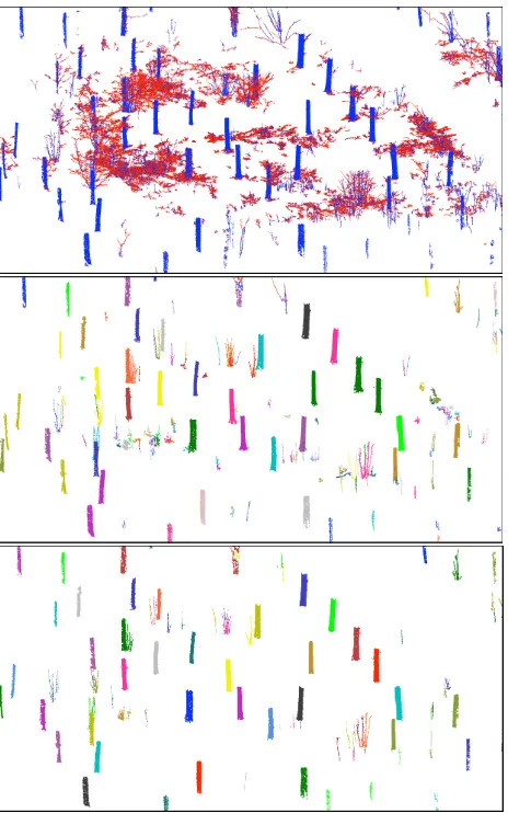
2.5.1 Locating stems and their bases The extraction starts by locating the stems. First the ground level is defined by parti-tioning the cover sets into 0.25 m horizontal squares and defin-ing the ground level for each square as the lowest z-coordinate in its 5x5 neighbourhood. The ”height” for each square is de-fined similarly. Next the surface normals of the cover sets up to 3 m above the ground are determined as the smallest principal component. The sets whose angle between the normal and the z-direction is overαare selected as the most likely sets from stems (see the top of Fig. 2). We setαto 70 degrees. From these sets, with approximately horizontal normals, connected components are determined and components with overκsets are selected as potential stems (see the middle of Fig. 2). We set
κ= ceil[ 0.2
(1.4d1)2] (2)
whereceilis the rounding to the nearest bigger integer. These components are now very probably part of the stems, but multiple components can be from the same stem. The components whose centres are horizontally closer thanδto each other are combined into one. We setδto 20 cm. Finally the bottom 25 cm of each component is removed as the potential layer containing ground, understory, and buttresses. Those components that still have at leastκsets and whose vertical height is overλ= 1m are selected as the final locations of the stems (see the bottom of Fig. 2).
Next the bases of the stems are determined. A cylinder giving the approximate stem diameter is fitted for each stem component. The component is then restricted to its bottom 70 cm and is ex-panded downwards with neighbours, and only sets with normals overαare accepted. After each expansion the cylinder is fitted again. The expansion is stopped when 1) the diameters of the cylinders are almost equal, or 2) the diameters are very different, or 3) the bottom is under 10 cm from the ground level. Then the bottom 50 cm of the expanded component is the base of the stem (see the top of Fig. 3). The above process has four parameters;
α,κ,δ, andλ, but it is insensitive to quite large changes in their values as shown in the section 2.7.
Figure 2. Locating stems. Top: ”Stem-like” cover sets whose normals are nearly horizontal (blue) and the other cover sets (red) of the bottom 3 m. Middle: The initial components of ”stem-like” sets. Bottom: The final stem components which define the stems.
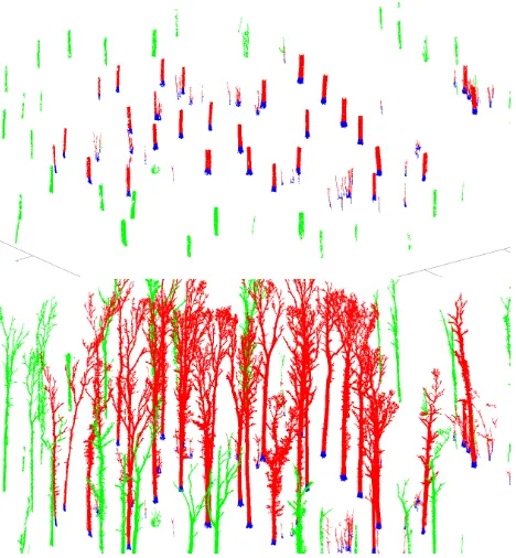
Because the extraction is based on segmentation, it is essential to segment also trees whose stem is outside but near the plot’s boundary. Therefore all stems whose distance from the plot’s centre is less thanRplot+ 10m are segmented (the red stems in Fig. 3) and all sets further thanRplot+ 15m are classified as other (the green stems in Fig. 3).
2.5.2 Classifying sets The next step is to classify every cover set either as tree or other. We begin by expanding the stem com-ponents upwards to determine the stems approximately (see the bottom of Fig. 3). We want approximate stems for robust tree extraction and the determination of initial ground and understory sets. To prevent an expansion too much downwards along branches or into understory or ground, the expansion is restricted to neigh-bours that are, e.g., under 50 cm from the current highest set. Due to occlusion this expansion may stop before the top of the tree. In such a case the nearest sets above the current top of the expansion are connected to the top and the expansion is continued until the top of the tree is reached.
The ground and understory sets are next defined as the non-stem sets in the 1-m layer above the ground level. These sets are then expanded as much as possible with the neighbours. At this point every set is classified as tree (stem) or other (ground and under-story), or is not classified (see Fig. 4).
Figure 3. Approximate stems and their bases. Top: The stem components of Fig. 2 are expanded downwards and their bottom part (blue) is selected as the base. Green components are too far away from the plot’s centre. Bottom: The stem components are expanded upwards to define the stems approximately.
Figure 4. Classification of sets. Tree (red) and other (green) ex-panded as much as possible. Purple points are the non-classified sets which will be classified either as tree or other.
to tree or other sets. First we expand the tree sets into unclassi-fied sets as much as possible. If there still are unclassiunclassi-fied sets, then we connect them to either class. We determine the connected components of the unclassified sets and using the cubical parti-tion, with initially about 20 cm cubes, we check if each compo-nent has in its neighbouring cubes tree or other sets. A compocompo-nent is connected to the closest tree or other set. In this process we first connect the nearest components, which then expand the tree and other sets step-by-step. If there are gaps so large that some com-ponents cannot be found in the neighbouring cubes of expanding tree or other sets, then we increase the size of the cubes as long as needed.
2.5.3 Segmentation of trees For the extraction of individual trees from the tree sets we use the segmentation method presented in Raumonen et al. (2013). We start from one of the bases of the stems and expand it step-by-step with neighbours. If the ex-panding “front” becomes disconnected, then there may be a bi-furcation, in which case a new branch basis is defined and further expansion into that branch is prevented. The stem is defined by expanding it as much as possible, after which the same is done for the other stems. The process continues case-by-case from the bases of the first-order branches, and so on from the second-order
Figure 5. Segmentation of the tree sets. Stems are in blue, 1st-order branches in green, 2nd-1st-order branches in red, etc.
branches, etc., until every tree is segmented.
This initial segmentation may have problems: segments stop too early, or take wrong turns at bifurcations, or small segments could be part of bigger segments. We try to make some modifications to make the segmentation more correct, i.e., such that each seg-ment corresponds to a real stem or branch without child branches. First we try to make the segments as long as possible, to correct the early stops or wrong turns. For each segment we select all the segments that can be traced back to it with the parent relation of the segments. Then we calculate the distances from the tips of these segments to the base of the current segment. If the furthest tip of these segments is farther than the tip of the current segment is from its base, we modify the segments and their parent-child re-lations so that the current segment continues without bifurcations to the furthest tip. The modification conforms to the branching order, i.e. first the stem, then the first-order branches, etc. For stems and first-order branches we use restrictions on the length vs. distance ratios making the segments nearly straight. Fig. 5 shows an example of the final segmentation of the point cloud, and the middle of Fig. 1 shows the extracted individual trees in-side the plot.
There can be some problems in the resulting tree extraction. Due to occlusion, some tree parts may be quite far away from any other tree parts, and in our process this part is then connected to the closest tree part, which may not be the right one. In these situations, based on the distances from the stems and other in-formation, one can try to estimate the likelihood that the part is connected to the right tree. We have not applied such methods in practice. Furthermore, two segments from different trees may touch each other, and because of their generation process, there is no guarantee that this connecting place is accurate. One frequent reason for this is that there is an erroneous connection made be-tween tree parts and one tree reaches the other over a big gap. If this is the case, then we can expand through neighbours from the enjoining location into both trees and see if there are big gaps between neighbouring cover sets (see Fig. 6).
Figure 6. Tree extraction correction. Left: Blue denotes the meet-ing of two trees (red and green). Right: The expansion from the meeting place into the green tree is stopped earlier than the ex-pansion into red tree because of a big gap and thus this expanded part is added to the red tree.
into cover sets: the base is the first layer, the second layer consists of its neighbours, etc. The ”thickness” of the branches and stems are estimated as the number of cover sets in the layers 2 - 6. The relative size of the sets at the base of a branch is the quotient of the thicknesses of the branch and stem. Furthermore, the size of the sets decreases along the branch from the base to the tip to the user-defined minimum.
2.6 QSM of individual trees
From the tree extraction we have the point clouds of individual trees and the relative size of the cover set for every point, based on the likely sizes of local details. For each tree the QSM is reconstructed separately with the following steps. First generate a random cover with a varying set size. Next define the base of the stem as the bottom 20 cm layer of the point cloud and update the neighbour relation to make the whole tree connected. Then segment the tree into its stem and branches. Finally fit cylinders to the segments.
All steps until the cylinder fitting are similar to those described in the tree extraction phase. The cover parameters are r2 and
d2, which give the maximum set sizes, and f, which gives the fraction of the minimum and maximum set sizes. The local sizes are calculated from these parameters. For the oak plot we used the valuesd2 = 6cm,r2 = 6.6cm,n1 = 3,f = 0.25, and for the eucalyptus plot we used the larger valuesd2 = 8cm,
r2 = 8.8cm,n1 = 3, andf = 0.333. We always made five
QSMs per tree to estimate the inherent modelling variations due to the randomness in cover generation. Furthermore, if the DBH of the first QSM was under 80 % of the stem diameter used in the stem location process, then we progressively added 1 cm tod1
andr1until the DBH of the QSM is over the threshold.
The refining of the segmentation is exactly the same as explained above, but there are two additional steps at the end. First, very small segments are removed if they do not have child segments and if their distance from the parent is not much more than the radius of the parent. Second, often some part of the real base of a segment is left to the parent segment forming quite large ledges. These ledges can make cylinder fits at their location too large. Thus we try to remove these ledges partly or entirely (see Appendix of Raumonen et al. 2013). The refining process can substantially reduce the number of segments and the maxi-mum branching order so that the final segmentation usually cor-responds well to the real branching structure.
2.6.1 Cylinder fitting In the last step of the QSM reconstruc-tion, cylinders are fitted to the segments. Here we introduce an-other input parameterl, which controls the relative length of the cylinders, i.e., the ratio of the length and radius of the cylinder. Shorter cylinders can better approximate the local size and cur-vature of the branches but, especially with small branches, noise, an incomplete point cover, etc., can make them also more sensi-tive to errors. Longer cylinders are less likely to be affected by such factors, but they can be too large due to the curvature or the tapering of the branch. For both plots we used the valuel= 3.
The reconstruction proceeds according to the branching order; first the stem, then the first-order branches, etc. Each segment is first divided into subregions so that their approximate relative length is close to l. The radius is estimated as the median of the point distance from the approximated axis, which in turn is estimated as the vector from the region’s base to the region’s top.
Cylinders are fitted to the regions by least squares. The fitting is renewed with the farthest points from the cylinder surface re-moved as outliers. We accept the fitted cylinder if i) the radius is under three times the initial estimate, ii) the angle between the initially estimated axis and fitted axis is under 35◦, and iii) the mean absolute distance to the cylinder’s surface is smaller than the initial estimate for the radius.
The radii of the cylinders along the branch are corrected locally by imposing maximum and minimum taper curves. Details for this are presented in Calders et al. (2014). Finally the starting points are also improved to close possible gaps between cylinders by extending the starting point into the plane defined by the parent cylinder’s end circle.
2.7 Sensitivity analysis
In this kind of reconstruction there usually are some parameters whose values must be given and which can affect the final results greatly. A useful and reliable method should not be sensitive to the exact values of these parameters, and a robust method should work even with relatively large changes in the values.
The important parameters in the tree extraction step are the cover parameterd1andα,κ,δ, andλused in the stem locating
pro-cess (see Sec. 2.5.1). Table 1 shows the values given to these parameters. Forκthe value in the table is the numerator in Eq. 2. Furthermore, due to randomness, the covers for different runs are always different, which can have effects on the stem locating. Thus we have 6 variables and we ran the stem locating with all possible 1296 combinations for the oak plot. We counted the number of big stems found inside a 20-m circle and compared it to the visually determined reference value. In all cases all refer-ence stems were found inside the circle, and only one referrefer-ence stem was missing in a few cases outside the circle. Thus the stem locating, at least for the oak plot, seems to be very robust and not very sensitive to relatively large changes in different parameter values.
Parameter Values Units
Cover set diameterd1 8; 10; 12; 14 cm
Number of covers 4
”Normal angle”α 60; 70; 80 degrees ”Component size”κ 0.1; 0.2; 0.3
”Component distance”δ 10; 20; 30 cm ”Component length”λ 0.5; 1; 1.5 m
Table 1. Parameters in the sensitivity analysis of stem locating.
Other important parameters ared2 and lfor reconstructing the
et al. 2014) and we are publishing soon a more detailed analysis on these, so we do not present a detailed analysis here. We only mention here that the resulting QSM and particularly its branch volume can be somewhat sensitive to the chosen values ofd2and l. Usually the volume increases as we increase the values of these parameters, so they should be quite small. On the other hand, making them too small makes the results unstable.
3. RESULTS
3.1 The oak plot
We made five different covers for the tree extraction part (d1= 8
cm,r1 = 9cm,n1 = 3) and for each of these cases we made
five different QSMs per extracted tree (d2= 6cm,r2= 6.6cm,
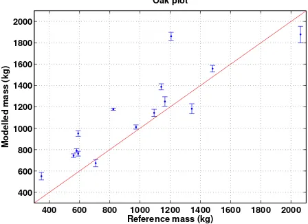
n2 = 3,f = 0.25). From the modelled volume we computed the dry masses using the density and the reference dry mass com-puted from the empirical relation given in Eq. 1 using the DBH of the QSMs. Fig. 7 shows the average modelled masses from five different QSMs for each tree for one of the extraction cases and compares them to the reference values (the error bars show two standard deviation of the means from the five QSMs). The average relative absolute error for the five tree extraction cases varies from 23.7 % to 25.5 %, and the total plot level biomass overestimation varies from 15.3 % to 18.8 %. All the 15 trees inside the plot were extracted and modelled for each case. The total modelling time for filtering, tree extraction, and one QSM per tree was about 1 h 40 min for each case (MATLAB, Mac-Book Pro, 2.8GHz, 16GB). With five QSMs per tree, the total modelling time was about 4 h for each case.
400 600 800 1000 1200 1400 1600 1800 2000
400 600 800 1000 1200 1400 1600 1800 2000
Oak plot
Reference mass (kg)
Modelled mass (kg)
Figure 7. Comparison of modelled individual tree masses for the oak plot. The red line is the 1:1 line, the blue dots are averages and the error bars denote two times the standard deviation com-puted from 5 different QSMs.
3.2 The eucalyptus plot
We used one cover for the tree extraction part (d1 = 10cm,
r1= 12cm,n1= 3) and made five QSMs per tree (d2= 8cm,
r2 = 8.8cm,n2 = 3,f = 0.333,l= 3). From the modelled
volume we computed the dry masses using the density and the reference dry mass was computed from destructively measured fresh weight for 27 trees. Fig. 8 shows the average modelled masses from five different QSMs for each tree and compares them to the reference values (the error bars show two standard devia-tion of the means from the five QSMs). Fig. 9 shows the tree seg-mented point cloud and QSMs. From visual inspection we can say that every tree inside the plot was extracted and modelled.
However, in the plot there are some multi-stem trees, whose stem bifurcates very close to ground. Most of these were extracted as single trees, such that one of the stems was segmented as the stem and the others as big branches. A few reference trees were multi-stem trees, where the reference mass was measured for each multi-stem. In these cases we added the reference masses together to give the reference for the one modelled tree. The average relative abso-lute error was about 28.5 % and the error in the total biomass of the reference trees was about 8.5 %. The total modelling time for filtering, tree extraction, and one QSM per tree was about 2 h 40 min (MATLAB, MacBook Pro, 2.8GHz, 16GB). With five QSMs per tree, the total modelling time was about 9 h.
0 500 1000 1500 2000 2500 3000
0 500 1000 1500 2000 2500 3000
Eucalyptus plot
Reference mass (kg)
Modelled mass (kg)
Figure 8. Comparison of modelled individual tree masses for the eucalyptus plot. The red line is the 1:1 line, the blue dots are av-erages and the error bars denote two times the standard deviation computed from 5 different QSMs.
4. DISCUSSION
The results show that the automatic tree extraction and QSM re-constructions are fast, robust, and accurate. The computation time for the filtering, tree extraction, and QSM reconstructions was altogether a few hours for both plots.
All the trees inside the oak plot were found and correctly ex-tracted except for a few small errors with some small branches. In the case of the eucalyptus plot all the trees were also extracted, but for some multi-stem trees there were bigger errors for sepa-rating the trees correctly, which appears in Fig. 8 as bigger errors and error bars. The heuristic stem location process was shown to be robust and insensitive to the four parameters used in the pro-cess as quite large changes in the parameter values did not affect the results. We used two completely different plots and scanners, and different scanning resolutions, which further corroborates the generality and robustness of the method.
The computed tree and plot level biomass were close to the ence values. Taking into account all the uncertainties in the refer-ence measurements, such as the wood density and dbh measure-ments, it is possible that the differences could be even smaller. In Calders et al. (2015) the same eucalyptus plot was modelled with the same QSM method; however, some details may have been dif-ferent, the tree extraction was not automatic, and different cover sizes were used. Their modelled biomass results were similar to the ones obtained here, as expected.
Figure 9. The extracted trees (top) and their QSMs (bottom) for the eucalyptus plot.
visibility would be poorer and we can imagine forest plots with much more understory and higher stem density. Plots that have lots of dissimilar tree species can be also challenging as different modelling parameters may be optimally suited for each species. These more challenging cases need more testing, validation, and further method development. However, these two plots can still be used for further testing and validation, and for example the multi-stems of the eucalyptus plot require modification to the al-gorithm to recognise them as separate trees, if needed.
In future, and to some extent already, the scanning is possible to do with mobile scanners, which means that large forest areas can be scanned more quickly and comprehensively. Our method is a good starting point for measuring the forest structure from these big data sets as the method scales up easily.
5. CONCLUSIONS
In this paper we have presented the first method that automati-cally extracts and reconstructs the volumes and 3D structures of all the individual trees in massive TLS point clouds. The method is a development of our earlier published method extracting and reconstructing a single tree from point cloud data. With two dif-ferent types of plots and two difdif-ferent scanners, we have shown that the method is accurate, robust, and fast.
Automatic tree extraction has been a big bottleneck for the large-scale use of TLS and reconstruction methods for estimating tree biomass and structure. We have demonstrated here that automatic and nondestructive biomass and structure estimation is possible in certain types of forests. Considerable further development is
still needed, but this method opens up numerous possibilities in the remote sensing of forests and their applications.
ACKNOWLEDGEMENTS
This study was financially supported by the Academy of Finland projectModelling and applications of stochastic and regular sur-faces in inverse problemsand the Finnish Centre of Excellence in Inverse Problems Research.
REFERENCES
˚
Akerblom, M., Raumonen, P., Kaasalainen, M., and Casella, E. 2015. Analysis of geometric primitives in quantitative structure models of tree stems. Submitted toRemote Sensing.
˚
Akerblom, M. 2014. 3D forest information.
www.youtube.com/watch?v=wANRdliE1zQ&spfreload=10
Calders, K., Armston, J., Newnham, G., Herold, M., and Good-win, N. 2014. Implications of sensor configuration and topogra-phy on vertical plant profiles derived from terrestrial lidar. Agri-cultural and Forest Meteorology, 194, pp. 104-117.
Calders, K., Newnham, G., Burt, A., Murphy, S., Raumonen, P., Herold, M., Culvenor, D., Avitabile, V., Disney, M., Armston, J., and Kaasalainen, M. 2015. Non-destructive estimates of above-ground biomass using terrestrial laser scanning.Methods in Ecol-ogy and Evolution, 6(2), pp. 198-208.
Dassot, M., Colin, A., Santenoise, P., Fournier, M., and Constant, T. 2012. Terrestrial laser scanning for measuring the solid wood volume, including branches, of adult standing trees in the forest environment. Computers and Electronics in Agriculture, 89, pp. 86-93.
Eysn, L., Pfeifer, N., Ressl, C., Hollaus, M., Grafl, A., and Mors-dorf, F. 2013. A Practical Approach for Extracting Tree Models in Forest Environments Based on Equirectangular Projections of Terrestrial Laser Scans.Remote Sensing, 5(11), pp. 5424-5448.
Hackenberg, J., Morhart, C., Sheppard, J., Spiecker, H., and Dis-ney, M.. 2014. Highly Accurate Tree Models Derived from Ter-restrial Laser Scan Data: A Method Description. Forests, 5(5), pp. 1069-1105.
Hopkinson, C., Chasmer, L., Young-Pow, C., and Treitz, P. 2004. Assessing forest metrics with a ground-based scanning lidar. Cana-dian Journal of Forest Research, 34(3), pp. 573-583.
Kaasalainen, S., Krooks, A., Liski, J., Raumonen, P., Kaartinen, H., Kaasalainen, M., Puttonen, E., Anttila, K., and M¨akip¨a¨a, R. 2014. Change Detection of Tree Biomass with Terrestrial Laser Scanning and Quantitative Structure Modelling.Remote Sensing, 6(5), pp. 3906-3922.
Maas, H. -G., Bienert, A., Scheller, S., and Keane, E. 2008. Automatic forest inventory parameter determination from terres-trial laser scanner data.International Journal of Remote Sensing, 29(5), pp. 1579-1593.