Gasoline demand and car choice:
estimating gasoline demand using
household information
Hilke A. Kayser
UHamilton College, 198 College Hill Road, Clinton, NY 13323, USA
Abstract
In recent years, calls for carbon taxes as a policy tool to combat global warming have kept a discussion of the price and income elasticities of gasoline demand alive. To date, gasoline demand elasticity estimates are almost exclusively based on aggregate data that are subject to aggregation problems and make distributional concerns impossible to address. By using
Ž .
household-level data from the Panel Study of Income Dynamics PSID and imputed fuel efficiency measures and gasoline prices, I estimate household demand for gasoline and the corresponding price and income demand elasticities. An attempt is made to include data on the car stock in the estimation since car-portfolio and gasoline demand decisions are closely related. Empirical results from a selection corrected gasoline demand regression suggest low short-run price and income elasticities and clear differences in gasoline demand across the population. These results suggest that a gasoline tax is not likely to result in large decreases in gasoline consumption while potentially imposing hardship on identifiable segments of the population.Q2000 Elsevier Science B.V. All rights reserved.
JEL classification: H2; Q41
Keywords:Gasoline consumption; Energy; Price elasticity
1. Introduction
Understanding the determinants of gasoline demand has been of interest to economists for almost three decades. Initially, studies mainly addressed concerns
U
Tel.:q1-315-859-4234.
Ž .
E-mail address:[email protected] H.A. Kayser
0140-9883r00r$ - see front matterQ2000 Elsevier Science B.V. All rights reserved. Ž .
about the availability of depletable resources and national security concerns raised by the oil supply shocks of the 1970s. Lately, studies increasingly address the various environmental consequences of gasoline consumption particularly with respect to the emission of greenhouse gases. A large number of studies have produced greatly varying estimates of the price elasticity depending on the
specifi-cation and the data used.1Almost all of the studies use data at the aggregate level
for reasons including the limited nature of data at the household level. It is well known that aggregate data may not be appropriate for an estimation of household responses to higher gasoline prices because of aggregation problems. Thus, the effects of higher gasoline prices on the demand for gasoline by households in the United States are still not well understood. The effectiveness and equity of a number of current policy suggestions depend on a clear understanding of private driving and the responsiveness of gasoline demand to income and price changes, warranting a further investigation of household demand for gasoline.
In this paper, I provide estimates of the demand for gasoline and the associated demand elasticities by using household level data from the Panel Study of Income
Ž .
Dynamics PSID . The PSID contains information about households’ annual miles
Ž .
traveled. Some standards by the Environment Protection Agency EPA for regu-lating tailpipe emissions of pollutants such as nitrogen oxides, carbon monoxide
and hydrocarbons are set per mile and tend to be directly related to miles driven.2
However, the emission of other pollutants } most notably carbon dioxide } is
directly related to gasoline consumption, not miles driven. In order to estimate the gasoline consumption we need to account for systematic differences in the fuel efficiency of the car fleet across the population. I therefore impute
household-Ž .
specific fuel efficiencies using data from the Survey of Consumer Finances SCF and information from the EPA. Gasoline demand is then obtained by dividing each household’s miles traveled by the household’s fuel efficiency estimate.
Estimating gasoline demand using household level data rather than aggregate data provides estimates that reflect more closely how individual consumers respond to changes in gasoline prices or household income, while allowing specific charac-teristics of a household to affect the demand for gasoline. As we will see, a household’s burden from higher gasoline prices is closely linked to observable characteristics of the household.
Besides using new and to a certain degree richer data sources, an important contribution of this research is the inclusion of data on the car stock. Since
1
For excellent surveys of the existing literature and the estimated price and income elasticities see Dahl
Ž1986 and Dahl and Sterner 1991 .. Ž .
2 Ž . Ž .
consumers receive utility from the transportation services that gasoline in combina-tion with an automobile determine, gasoline demand is an indirect demand. Car-portfolio decisions and gasoline demand decisions are therefore related. Previ-ous work using hPrevi-ousehold data to estimate gasoline demand has taken the households’ car stock as given, focusing only on short-run responses to price changes in the form of reduced miles driven. It is of interest, however, to allow for changes in the car stock to affect the demand for gasoline. Though the data at hand does not provide much information about the car stock, a household’s decision to own a car or not will be included in the specification.
In Section 2, I discuss the conceptual framework and the estimation methods used in the empirical work before describing the data. Estimation results for gasoline demand and miles traveled are presented and discussed in Section 4. The paper ends with a concluding summary.
2. Conceptual framework and empirical methods
In this paper, gasoline demand and the demand for automobiles are modeled as a joint decision. Gasoline demand as a function of the price of gasoline is a consumer choice decision that in principle is made simultaneously with the con-sumer’s choice about the car portfolio. Similarly, the choice of car hinges on the household’s need for transportation services provided uniquely or most cheaply by a car. Two specification issues follow. First, the unit of observation in the empirical work is the household since driving is inherently a household decision. Second, the underlying consumer choices suggest the simultaneous estimation of two related
Ž .
decisions by estimating a a discrete choice model for the automobile portfolio; Ž .
and b a continuous gasoline demand function that is conditional on the auto-mobiles owned.
A small number of studies have used household-level data to investigate gasoline
3 Ž .
demand over the past two decades. Archibald and Gillingham 1980 estimate
households’ gasoline demand in the United States using the 1973r1974 Consumer
Ž .
Expenditure Survey CES , a five-quarter panel data set. In their analysis, Archibald and Gillingham explicitly estimate the short-run demand for households living in
Ž .
23 larger Metropolitan Statistical Areas MSAs . Gasoline consumption is calcu-lated as the ratio of the reported gasoline expenditures divided by an average gasoline price from the Bureau of Labor Statistics for the 23 MSAs. Archibald and Gillingham’s price elasticity estimates are problematic because their dependent variable is measured with error. As they point out, the gasoline prices used to deflate gasoline expenditure and whose coefficients give rise to the estimated price elasticity are average gasoline prices. A household’s gasoline consumption is thus measured with error, and this error is obviously related to the price variable in the
3 Ž . Ž .
vector of regressors, leading to biased estimates. The income elasticity is also somewhat problematic since Archibald and Gillingham use total expenditures as a proxy for lifetime income. Annual expenditures have been shown to be a poor
Ž .
proxy for permanent income Hall, 1978; Menchik and David, 1982; Zeldes, 1989 such that the expenditure elasticity may not give a clear indication of the income elasticity of gasoline demand.
Ž .
In another relevant study, Mannering and Winston 1985 use household data to simultaneously estimate automobile choice and usage. Price elasticities of the
demand for miles tra¨eled are estimated in the process of estimating households’
demand for specific automobile attributes, and the importance of brand prefer-ences on the vehicle selection. For the time period between January 1979 and June
1980 they estimate a short-run price elasticity of y0.228 and an insignificant
short-run income elasticity of 0.049.
In this paper I build on previous work, using richer household data to simultane-ously estimate the binary decision about whether or not to own a car, and of the
continuous demand for gasoline.4 The underlying model best derives gasoline
consumption from a household production of transportation services. Together with the household’s automobile stock and time, gasoline enters as an input into the production of the economic good of transportation services. This leads to two equations. First it gives rise to an indirect demand for gasoline that depends on the household’s economic situation, household characteristics that influence the taste or need for transportation services, car characteristics as captured by the fuel efficiency of the car fleet, and prices. Second, it gives rise to a binary choice equation that relates the household’s car ownership to household characteristics, the household’s economic situation, and prices.
For the gasoline demand equation, a Box]Cox test does not provide conclusive
evidence as to the use of a log-linear specification or a linear one. Likelihood ratio tests present no preference for either a log-linear specification or a linear
specifi-cation.5 For ease of comparison, this paper will thus follow the log-linear
specifica-tion used by Archibald and Gillingham. The estimated equaspecifica-tion for the short-run demand of gasoline is as follows:
2
where ln g is the natural logarithm of gasoline consumption which is calculated
dividing reported number of miles by the estimated fuel efficiency of the
house-4
Unfortunately, the data are not rich enough with respect to car stock information to allow the estimation of a more structural model.
5
Ž .
hold’s car fleet and thus includes car characteristics, ln p is the logarithm of the
Ž . Ž .2
price of gasoline, ln m is the natural logarithm of income, ln m is the square of
Ž . Ž .
this quantity, ln pln m is an interaction term between the logarithm of income
and the logarithm of price, andWj is a vector of dummy variables to account for
taste differences.6
Included in the specification is an interaction term between income and the price of gasoline, following Archibald and Gillingham. By including the interaction term, I allow the price elasticity to vary across the income distribution. Poorer households who drive tend to spend a larger share of their income on gasoline and thus gasoline price changes have a larger impact for these households. Though it is possible that the relatively larger impact on their income makes the less well off more responsive to price changes, the fact that gasoline expenditure is such a large component of their overall expenditure may also be an indication that poorer households have very little choice in the amount of driving. It is probably fair to assume that the amount of driving they undertake, even though it imposes a large burden on them economically, must be necessary driving and cheaper than any available alternative, such as flying, taking the train or a bus. Wealthier households have less of a need to respond substantially to price changes, but they have more of an ability to do so. The price elasticity may therefore vary across the income distribution. For similar reasons, the income elasticity may also vary with the level
of prices.7
The automobile choice equation is discrete with the following general form:
K
X
U Ž .
Ci sg0qg1piqg2miqg3pciq
Ý
gkWi kq¨i'Zigq¨i 2 ks4where CU is the unobserved car ownership demand variable which takes on the
value one if the household owns at least one car, and zero if not, pci is the
estimated price of a car for household i, and Wi k is a vector of household
characteristics to account for different preferences in the demand for cars. In the empirical model I want to account for the fact that households may have a positive demand for gasoline but report no gasoline demand because they do not own a car, i.e. that car-ownership and gasoline consumption decisions are made jointly. This suggests using a two-stage estimation approach that was first discussed
6
Appendix A presents a discussion of biases from measurement error in the dependent variable of the sort that we would expect for the imputed gasoline demand variable in this study.
7
Ž .
by Heckman 1976 and is known as the Heckman selection correction model.
Gasoline demand is only observed when the household owns a car. Assume that «i
andnihave a bivariate normal distribution with zero means and correlation r. For
identification,su2 is normalized to one. Then the expected gasoline demand can be
expressed as:
and the demand for gasoline becomes:
Ž X .
In the Heckman selection correction specification, a Probit model is used for the
car ownership equation to obtain an estimate for the selection correction term li.
An ordinary least squares regression for the gasoline demand equation which includes that estimated selection correction term will lead to consistent estimates
for the coefficients,b, even in the case where the error terms are correlated.
For identification of the parameters in the two equations, one of two conditions must hold. Either the error terms have to be uncorrelated, or if the error terms are correlated, there has to be at least one variable in the vector of explanatory
variables in the car choice equation, W, that is not included in the vector of
Ž
explanatory variables in the gasoline demand equation, X Maddala, 1983, pp.
.
231]234 . I include an imputed average price of cars for each state. The price of a
vehicle should affect the likelihood of owning a car without having an effect on the Ž .
amount of driving. Given the specification in Eq. 4 I can determine the short-run elasticities as follows:
where m is the mean of average income and p is the average gasoline price in
the sample.
3. Data
To estimate the gasoline demand and car-ownership decisions I will use
house-Ž .
characteristics of the car fleet that travels the roads in the United States. However, data from 1981 are the most recent data for one year in which gasoline prices were changing rather substantially. The year 1981 is the last year of a period of substantially fluctuating prices that followed the oil supply shocks of the late 1970s. Ever since 1981, gasoline prices in the United States have fallen gradually in real terms. The 1981 data will therefore predict household responses to more substan-tial increases in the price of gasoline through a carbon tax or any other form of gasoline tax more accurate than would estimates from more recent data.
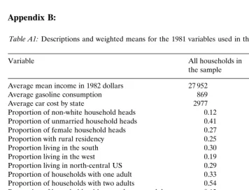
The PSID is a panel data set that was started in 1968 with approximately 5000 American households. Since 1968 the PSID has collected data annually from the households in the original sample as well as from any new household that was formed by members of the original families. Each sampled household responds to approximately 2000 questions. Table A1 in Appendix B presents means and standard deviations for the variables that enter the empirical model. The list of explanatory variables includes family composition dummies since one would expect households with a larger number of adults to drive more, while households with children may both require additional transportation services and drive less by staying more in the vicinity of the home. Dummy variables indicating whether the household is a one-adult household or one with more adults, and indicating whether the household has no children, one child or several children are thus part of the list of independent variables.
Also included are a number of demographic variables that serve as proxies for unobservable taste differences. Among these characteristics are ethnicity, gender,
age, marital status, and educational attainment of the head.8 These variables are
chosen because they either significantly affect gasoline demand in the works by
Ž . Ž .
Archibald and Gillingham 1980 , and Greening and Jeng 1994 , or because they are suggested as playing a role in household’s driving through differential treat-ment by automobile insurance policies.
The list of variables includes two variables that define the living environment of the household: whether a household lives in a rural environment, and whether public transportation is available for the household members to get them to work. It is likely that households living outside of metropolitan areas have different driving patterns than households who live in a large city or in the vicinity of a large city. Traveling distances are presumably longer for rural households, and house-holds in rural areas are assumed to drive larger, less fuel-efficient cars. Both higher annual mileage and lower fuel efficiency should increase the gasoline demand for
rural households.9
Economic factors are the household’s income, the price of gasoline for the household, and the employment status of the head of the household and the
8
Throughout the study I will use as head those designated head in the PSID. In a cohabitating couple this is generally the husband or male partner.
9
A dummy rather crudely classifies households as living in a rural setting if they do not live in or around
Ž .
spouse. The appropriate measure of household income is controversial. Since annual income may fluctuate substantially from year-to-year, annual income may not be the appropriate variable to measure a household’s well-being. Rather, according to Friedman’s permanent income hypothesis a better measure of a household’s income would be a measure that smoothes out annual fluctuation but
Ž
maintains variations across different stages in a household’s life-cycle Friedman, .
1957 . Accordingly, in the empirical work I use an income measure that averages household’s income over the 11-year period from 1976 to 1986, i.e. an average
centered around the reference year of 1981.10
Since the PSID does not contain information on gasoline prices, the prices used
Ž .
in this study are those developed by Chernik and Reschovsky 1992 . Using data from the Bureau of Labor Statistics, Chernik and Reschovsky assign average retail prices directly to households living in or around any of the 30 larger cities in the United States for which gasoline price data are readily available. The rest of the sample is stratified according to four US regions and three city sizes, resulting in 42 different prices net of taxes. For each state, these prices are adjusted to include local, state and federal taxes when these are applicable. Because of regional differences in the cost-of-living, all other prices are represented by a regional price index that reflects cost of living differences by state, as published by Fournier and
Ž .
Rasmussen 1986 for the year 1980.
The PSID also does not contain information on gasoline consumption or on the gas mileage which could be used to estimate households’ gasoline consumption. Consequently, prior studies have calculated each household’s gasoline consumption by dividing the reported miles by the average national fuel efficiency. However, this is a crude measure that ignores any variation in the fuel efficiency of car fleets across the population. In this study I adopt the following procedure to estimate gas
Ž .
mileage. Using the 1983 Survey of Consumer Finances SCF and the annual Gas Mileage Guides for New Car Buyers from the Environmental Protection Agency
Ž1974]1986 , I impute household specific gas mileage.. 11 The Survey of Consumer
Finances contains information on the number of cars as well as the make, model, and vintage of the first three cars in the household. I assign the fuel efficiency values for each make, model, and year of a car from the Gas Mileage Guide to the corresponding cars in the SCF and take a simple average across the cars in a household to arrive at an average fuel efficiency value of the household’s car fleet for all households in the SCF. In a second step I run an ordinary least squares
Ž .
regression of the imputed miles per gallon mpg , on a vector of explanatory
variables, X, that includes household income, gender, ethnicity, and age of the
household head, employment information, and information about the residential location of the household. The coefficients from the regression using data from the
SCF, b83, SCF, are used to calculate predicted fuel efficiency values for each
household in the PSID according to the following equation:
10
Not all households are part of the survey for all 11 years, in which case the average is calculated from the years that are available.
11
X Ž .
mpg83 ,PSIDsb83,SCFX83,PSID 7
Table A2 in Appendix B shows the coefficients and standard errors of the mpg
regression from which the coefficients b83,SCF are taken to impute fuel efficiency
Ž .
value for households in the PSID according to Eq. 7 . Using this more disaggre-gate measure of fuel efficiency, gasoline consumption is calculated by dividing the reported miles driven by the household-specific fuel efficiency. Since an imputed value from another data set is used, gasoline consumption will be subject to errors
in measurement that can lead to biased estimates.12
I also impute the estimated cost of a car using the SCF. The SCF contains information about the bluebook value for each of the first three cars in the household. For households with more than one car, the average car value was constructed. Regressing the average car value on household characteristics such as work status, household income, region of residence, number of adults, number of children, gender, race, and marital status in the SCF, I estimate coefficients that I can use to impute the average car value for all households in the PSID based on their household characteristic. Households that do not own a car thus also have a value of a car assigned to them. This value serves as a proxy for the amount of money a household with the given characteristics can be expected to spend were they to buy a car.
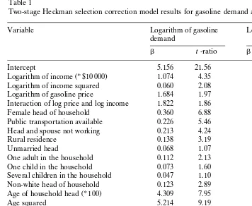
4. Estimation results
Table 1 shows the empirical results from the two-stage Heckman estimation of the model described above. The first three columns show the results using the natural logarithm of miles traveled divided by the imputed fuel efficiency as the dependent variable. The last three columns present results for a regression of the natural logarithm of the reported miles traveled on the same list of explanatory variables, also from a Heckman specification. The results from both Heckman
models show that the selection correction term,l, is statistically significant at the
5% significance level, indicating that households indeed self-select into the group of car-owning households, and that this self-selection has a significant influence on
gasoline demand and on the number of miles traveled.13
In this study I am mainly interested in the demand for gasoline so that the discussion of the results will primarily focus on the first set of regression results. The coefficients on the explanatory variables in the gasoline demand equation are mostly as predicted. Since the dependent variable is a natural logarithm of gasoline demand, the coefficients can be interpreted as percentage changes in gasoline
12
Refer to Appendix A for a more detailed discussion of the bias from measurement error.
13
Table 1
Two-stage Heckman selection correction model results for gasoline demand and miles traveled
Variable Logarithm of gasoline Logarithm of miles traveled
demand
Logarithm of income $10 000 1.074 4.35 0.917 3.19
Logarithm of income squared y0.060 2.08 y0.121 3.91
Logarithm of gasoline price 1.684 1.97 1.140 1.17
Interaction of log price and log income y1.822 1.86 y0.718 0.63
Female head of household y0.360 6.88 y0.331 5.61
Public transportation available y0.226 5.46 y0.245 4.86
Head and spouse not working y0.213 4.24 y0.306 5.20
Rural residence 0.138 3.19 0.101 1.95
Unmarried head 0.068 1.07 y0.115 1.48
One adult in the household y0.112 2.13 y0.072 1.17
One child in the household 0.073 1.60 y0.054 0.99
Several children in the household y0.047 1.10 y0.059 1.15
Non-white head of household y0.123 2.89 y0.227 4.53
U
Ž .
Age of household head 100 4.309 7.95 3.961 6.39
Age squared y5.214 9.19 y4.814 7.38
Household head did not finish high y0.090 1.38 y0.136 1.66
Household head has a high school y0.065 1.00 y0.099 1.23
Beyond high school, no advanced 0.038 0.61 0.017 0.22
Žselection correction term. y0.392 2.88 y0.584 3.77
N 4944 4944
consumption. Halvorsen and Palmquist 1980 show that the percentage impact of
the dummy variables on gasoline demand is eb
y1. Generally, eb
y1 and b tend
to be close in magnitude, but they do not have to be.14
The empirical results suggest that households headed by a woman consume approximately 30% less gasoline than households headed by a man, ceteris paribus. Though this value appears to be high, the reader should keep in mind that households with both male and female adults present during the interviewing period are coded as having a male head of household, leaving as female heads of household essentially only households with one or more female adults. Such female-only households are likely to be different in a variety of unobservable dimensions that I do not control for other than just their gender. Other findings
14
indicate that households with a non-white head of household consume on average 11.6% less gasoline than their white counterparts, and that age has a positive and significant effect on gasoline consumption though at a decreasing rate. Having both
the head and the spouse}if present }be unemployed lowers gasoline
consump-tion significantly as does having only one adult in the household.
The living environment has a significant effect on gasoline consumption. As predicted, living in the presence of good public transportation tends to significantly lower gasoline consumption by as much as 20%. On the other hand, living in a rural setting increases gasoline consumption. The level of education and the number of children in the household do not appear to significantly affect gasoline consumption. Though it is intuitively reasonable to assume that children affect a household’s driving pattern and car choice, it appears as though the various plausible behavioral responses to having children cancel each other out, leaving households with children with a demand for gasoline that is very similar to that of households who do not have children.
The coefficients involving income are also as expected. The results indicate that households with higher incomes tend to consume more gasoline but that the additional consumption comes at a decreasing rate. The estimated income and
Ž . Ž .
price elasticities are located at the bottom of the table. Recall from Eqs. 5 and 6 that the price elasticity for this specification is a function of average income, and the income elasticity is a function of both the price of gasoline and the average income. Evaluated at a mean average income of $28 667 and an average gasoline
price of $1.29, the estimated short-run price elasticity isy0.23 and the estimated
short-run income elasticity is 0.48.15A Wald test for joint significance of the two
coefficients involving the price of gasoline reveals that the coefficients and thus the price elasticity estimates are jointly marginally significant at the 10% significance level. A similar test for the income coefficients reveals that the income coefficients are significant at the 5% significance level.
The interaction term between the price of gasoline and income implies that the income elasticity is lower when prices are higher, and that the price elasticity is greater at higher levels of income. The coefficient confirms the suspicion that households with lower incomes do not respond as much to higher gasoline prices as wealthier households. As discussed earlier, it is not unreasonable to assume that households whose burden from gasoline expenditures is relatively high because of their low incomes are likely to have reduced their gasoline consumption to the amount that is necessary for them to get to work or to town, leaving little room to respond noticeably to higher prices. Though wealthier households may have less of an incentive to respond to higher gasoline prices, they are probably more able to do so because some of their consumption is less of a necessity.
Results from the regression of miles dri¨enserve to decompose the effects of the
15
explanatory variables on gasoline demand into effects on the quantity of driving and on the efficiency with which the miles were driven, as well as to make sure that the estimation results are reasonable and not an artifact from the imputed fuel efficiency measure. Regression results using reported miles driven as the depen-dent variable are fairly similar to those for gasoline demand. Households headed by a woman drive significantly fewer miles than households headed by a man, marital status and the number of children has no significant effect on miles driven, and education plays at best a marginal role in determining the amount of driving. Households who live in a rural setting tend to drive more miles, while access to public transportation lowers the amount of miles driven. Age affects miles driven positively but at a decreasing rate, and households with a non-white head or without work tend to drive fewer miles. Income has a positive effect on miles driven but at a decreasing rate. The income elasticity is significant and with a magnitude of 0.46 similar to the one estimated for gasoline demand.
A number of factors are different across the two regressions, however. Most importantly, the price coefficients and the price elasticity are not statistically
significant at all. Thex2-test for joint significance of the coefficients involving the
price of gasoline shows a significance level of 0.40. At least in the sample at hand, the price of gasoline has no significant effect on the number of miles households drive though it had a marginally significant effect on gasoline consumption. Households do not appear to respond to higher prices by reducing the amount of driving but rather by traveling the same miles more efficiently by shifting
transportation to the most fuel-efficient car in their fleet, or } in the longer run
} by replacing older and less fuel-efficient cars with newer ones.
Other noteworthy results from this comparison are that rural households not only drive longer distances but also do so in less fuel-efficient cars, and that households with a non-white head drive fewer miles while consuming less gasoline, suggesting that white households drive more but do so in more fuel-efficient cars. A very similar result holds for unemployed households when compared to house-holds where the head of household or the spouse are employed. Though the former travel approximately 30% fewer miles, they consume only 19% less gasoline.
In another attempt to see whether using the imputed fuel-efficiency measure may lead to bias because of errors in measurement, a separate regression was run using as the dependent variable the natural logarithm of gasoline consumption where gasoline consumption was calculated by deflating the miles driven by the national average fuel efficiency of 15.94 mpg. The results obtained are very similar to the results using miles traveled, with a significant income elasticity of 0.47. Again the price coefficients fail to be statistically significant with a significance
level of 0.38.16
16
5. Conclusions
The results from the empirical work in this study confirm that the price elasticity of gasoline demand is low in the short-run. The price elasticity found in this study is lower than the corresponding price elasticities found by Archibald and Gilling-ham, the only other study using household-level data to estimate a gasoline
demand equation. While the short-run price elasticity estimate is y0.23 when
evaluated at mean prices and mean income, Archibald and Gillingham estimate a
price elasticity ofy0.254 for households with one car andy0.376 for households
with several cars. Both studies indicate, however, that higher gasoline prices will not lead to a substantial reduction in the amount of gasoline consumed by households in the short-run.
Gasoline demand is calculated by deflating the reported miles traveled by the
imputed household-specific fuel efficiency. Estimating the demand for miles tra
¨-eled separately reveals a positive and highly insignificant price elasticity. If we
believe that the imputed household-specific fuel efficiencies capture some of the true variation in fuel efficiency across the population, then this result suggests that gasoline demand responds to changes in the price of gasoline mainly through adjustments in the fuel efficiency of the car fleet and not through an adjustment of miles traveled.
The estimated gasoline demand equation provides short-run income elasticity estimates of 0.49, and the miles traveled equation provides short-run income elasticity estimates of 0.48. In both cases the income elasticity is highly significant, and they are quite similar in magnitude. The magnitude is also in line with other
estimates of the short-run income elasticity.17 The fuel efficiency regression shows
that income is a significant explanatory variable for the fuel efficiency of a household’s car fleet, and Appendix C also shows a consistently positive relation-ship between income and fuel efficiency for each of the chosen subgroups. It appears that higher income allows households to purchase newer cars that will on average be more fuel-efficient because cars in 1981 are subject to the corporate fuel efficiency standards.
Finally, the empirical results show that there are clear differences in gasoline demand across the population. Households living in a rural setting and households with no public transportation available for travel to work will on average be affected more strongly by higher gasoline prices than similar households in an urban setting and with access to public transportation. Households whose head
andror spouse are working also consume significantly more gasoline. The working
poor who have to commute to work by car and have no access to public transporta-tion, for example, will be hurt more by raising prices than non-working poor who live off transfer programs. Information of this kind can be very valuable to policy makers who are interested in raising gasoline taxes for a variety of perfectly
17 Ž .
legitimate reasons but recognize the need for adequately compensating those who are economically disadvantaged and may be disproportionately affected by higher gasoline costs.
Future research in the direction of making the car choice equation richer appears desirable. I would assume that most responses to higher gasoline prices in terms of a household’s car fleet will not occur at the extensive margin but rather at the intensive margin. For example, households are likely to purchase more
fuel-ef-ficient cars when gasoline prices are high andthey are in the market for replacing
their car, and it is likely that households with several cars will shift some of the uses from the less fuel-efficient car to the more fuel-efficient one. Capturing effects on gasoline demand of these kinds of adjustments to price changes requires significantly more detailed information about a household’s car fleet than is available in the data used for this study.
Appendix A: Measurement error
The dependent variable in this paper is the gallons of gasoline a household consumed in the previous year. This variable is the ratio of the reported miles driven by the household divided by the imputed fuel efficiency measure. The fuel efficiency variable is measured with error and can thus be expressed as the true,
unobserved fuel efficiency value, mpgU, and the equally unobserved measurement
error,¨. The effect of the measurement error on the estimated coefficients can be
demonstrated using for simplicity a simple regression of gasoline consumption on
the price of gasoline. LetY be the logarithm of gasoline consumption. ThenY can
be expressed as:
miles miles U U
Ž . Ž .
Ysln
ž
/ ž
sln U/
(ln gallons yhsY yh A1mpg mpg q¨
The regression equation becomes:
U X Ž .
Y yhsX bq« A2
and the regression coefficients can be calculated as:
Ž . w x w x w x
cov x,y E xy yE x E y
bs s
Ž . Ž .
var x var x
wŽ U . x wŽ U . w .
E y yh x yE y yh E x
s
Ž .
w U x wŽ U . w .
The direction of the bias from a measurement error thus depends on the covariance between the unobserved error and the explanatory variable, i.e. the
w x w x
coefficient will be biased negatively if E hx )0 and negatively if E hx -0. The
magnitude of the bias will also be influenced by the variance of the regressor.
Appendix B:
Table A1:Descriptions and weighted means for the 1981 variables used in the regression model18
Variable All households in Car-owning
the sample households only
Average mean income in 1982 dollars 27 952 30 738
Average gasoline consumption 869 1015
Average car cost by state 2977 3090
Proportion of non-white household heads 0.12 0.09
Proportion of unmarried household heads 0.41 0.33
Proportion of female household heads 0.27 0.20
Proportion with rural residency 0.25 0.27
Proportion living in the south 0.30 0.30
Proportion living in the west 0.19 0.20
Proportion living in north-central US 0.29 0.29
Proportion of households with one adult 0.33 0.26
Proportion of households with two adults 0.54 0.60
Proportion of households with more than two adults 0.13 0.14
Proportion of households with no children 0.60 0.57
Proportion of households with one child 0.16 0.17
Proportion of households with several children 0.24 0.25
Proportion of households with head not working 0.27 0.21
Proportion with head with no high school degree 0.31 0.26
Proportion with head with high school degree 0.18 0.19
Proportion with head with additional education, no degree 0.32 0.34 Proportion with high quality public transportation 0.40 0.36
Head’s age 48 46
Number of observations 4944 3979
Table A2: Ordinary least squares regression of fuel efficiency using data from the 1983 survey of
Ž .
consumer finances dependent variable: miles per gallon
18
Variable b Standard error
Value of the house y0.0046 0.002
a Ž .
Number of cars y0.368 0.104
a Ž .
Two adults employed 0.665 0.208
a Ž .
No adult in household employed y0.889 0.298
Ž .
More than three children y0.960 0.514
Ž .
More than three adults 0.277 0.365
Ž .
Three adults y0.084 0.253
Ž .
One adult y0.099 0.353
a Ž .
Head has a college degree 1.637 0.223
a Ž .
Head went to college, no degree 0.906 0.234
a Ž .
Head did not complete high school y0.802 0.216
a Ž .
Head is Caucasian 1.621 0.492
a Ž .
Head is not Caucasian and not black 1.440 0.280
a Ž .
Head is male y0.342 0.165
Ž .
Head has never been married 0.392 0.429
a Ž .
Head own a house y0.357 0.215
N 3148
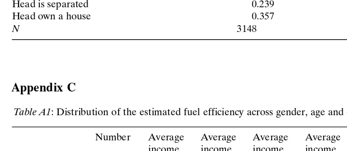
Appendix C
Table A1: Distribution of the estimated fuel efficiency across gender, age and ethnicity in the 1983 PSID Number Average Average Average Average Average Average
income income income income income income
10 000 10 000] 15 000] 20 000] 30 000] )40 000 15 000 20 000 30 000 40 000
Number 594 580 604 994 585 647
Male head 3189 15.38 15.58 15.61 15.92 16.21 16.47
Female head 815 15.90 15.93 16.23 16.35 16.55 16.15
White head 3640 15.91 16.14 16.21 16.25 16.41 16.56
Non-white head 364 15.56 15.20 15.09 15.23 15.48 16.66
Head age -25 337 16.10 16.37 16.37 16.62 16.89 16.49
x
Head age 25]44 2041 15.89 15.83 15.96 16.09 16.2 16.39
Head age 45]64 1156 15.68 15.40 15.40 15.63 16.14 16.59
Head age )64 470 15.54 15.43 15.30 15.60 15.87 16.14
Ž .
Table A1 shows the distribution of miles per gallon mpg across a few different demographic groups in the 1983 SCF. In all but the highest income bracket, households with a female household head drive more fuel-efficient cars than households with a male head, and households with a white head of household drive more fuel-efficient cars than households with a non-white head. Fuel efficiency of the car fleet tends to decrease with the age of the head while it increases with average income. These results and further results regarding the distribution across regions, education of the head of household, and rural or urban location coincide
Ž .19
with the results found by Greenlees 1980 . Since the distribution of the imputed
fuel efficiency in the 1981 PSID is similar to the one Greenlees finds in his study, it appears that at least some of the distributional differences in the fuel efficiency across different population groups have been captured correctly through the imputation.
References
Archibald, R., Gillingham, R., 1980. An analysis of the short-run consumer demand for gasoline using household survey data. Rev. Econ. Stat. 623]629.
Chernik, H., Reschovsky, A., 1992. Is the Gasoline Tax Regressive? Institute of Research on Poverty, Discussion Paper 980]992.
Dahl, C.A., 1986. Gasoline demand survey? Energy J. 7, 67]82.
Ž .
Dahl, C.A., Sterner, T., 1991. Analyzing gasoline demand elasticities: a survey. Energy Econ. 13 3 , 203]310.
Environmental Protection Agency, 1974]1986. Gas Mileage Guide for New Car Buyers. EPArFEA, Washington, DC.
Espey, M., 1997. Pollution control and energy conservation: complements or antagonists? A study of
Ž .
gasoline taxes and automobile fuel economy standards. Energy J. 18 2 , 23]38.
Fournier, G.M., Rasmussen, D.W., 1986. Salaries in public education: the impact of geographic
Ž .
cost-of-living differentials. Public Finance Q. 14 2 , 179]198.
Friedman, M., 1957. A Theory of the Consumption Function. Princeton University Press, National Bureau of Economics Research, Princeton, NJ.
Greening, L.A., Jeng, H.T., 1994. Lifecycle analysis of gasoline expenditure patterns. Energy Econ. 16
Ž .3 , 217]228.
Greenlees, J.S., 1980. Gasoline prices and purchases of new automobiles. South. Econ. J., 167]178. Hall, R.E., 1978. Stochastic implications of the life cycle-permanent income hypothesis: theory and
evidence. J. Pol. Econ. 86, 971]987.
Halvorsen, R., Palmquist, R., 1980. The interpretation of dummy variables in semilogarithmic equations.
Ž .
Am. Econ. Rev. 70 3 , 474]475.
Heckman, J., 1976. The common structure of statistical models of truncation, sample selection, and limited dependent variables and a simple estimator for such models. Ann. Econ. Soc. Measure. 5, 475]492.
Ž .
Hill, D.H., 1980. The relative burden of higher gasoline prices. In: Duncan, G.J., Morgan, J.N. Eds. , Five Thousand American Families } Patterns of Economic Progress, vol. 8. Institute for Social Research, Ann Arbor, pp. 87]413.
19
Holmes, J.W., 1976. The relative burden of higher gasoline prices. In: Duncan, G.J., Morgan, J.N.
ŽEds. , Five Thousand American Families. } Patterns of Economic Progress, vol. 4. Institute for Social Research, Ann Arbor, pp. 183]199.
Khazzoom, J.D., 1991. The impact of a gasoline tax on auto exhaust emissions. J. Pol. Anal. Manage. 10
Ž .3 , 434]454.
Maddala, G.S., 1983. Limited-Dependent and Qualitative Variables in Econometrics. Economic Society Monograph No. 3. Cambridge University Press, New York.
Mannering, F., Winston, C., 1985. Vehicle demand and the demand for new car fuel efficiency. Rand J. Econ. 16, 215]236.
Menchik, P.L., David, M., 1982. The incidence of a lifetime consumption tax. Natl. Tax J. 35, 189]203. Zeldes, S.P., 1989. Consumption and liquidity constraints: an empirical investigation. J. Pol. Econ. 97,